Yield variance is the difference between the standard yield specified and the actual yield obtained. In other words, the difference between actual yield of materials in manufacture and the standard yield (i.e. expected yield from a given standard input) valued at standard output price is known as materials yield variance. This variance is of great significance in processing industries, in which the output of one process becomes the input of the next process till the finished product is obtained at the final stage. The analysis of this variance helps effective control over usage. A low actual yield is unfavorable yield variance which indicates that consumption of materials was more than the standard. A high actual yield indicates efficiency, but a constant high yield is a pointer for the revision of the standard.
Material Yield Variance = Standard cost per unit (Actual yield – Standard yield)
i.e. SC p.u. (AY-SY)
Note: AY will never change. SY will calculate for actual mix of quantity as under:
New SY= Old SY x TAQ
TSQ
The yield variance may be caused by such factors as: defective methods of operation, sub-standard quality of materials purchased, lack of due care in handling, lack of proper supervision etc.
Illustration 1
For producing one unit of a product, the materials standard is:
Material X : 6 kg. @ 8 per kg., and
Material Y: 4 kg. @ 10 per kg.
In a week, 1,000 units were produced the actual consumption of materials was:
Material X : 5,900 kg. @ 9 kg., and
Material Y: 4,800 kg. @ 9.50 per kg.
Compute the various variances.
Solution:
Standard cost of materials of 1,000 units:
Material X: 6,000 kg. @ 8 48,000
Material Y: 4,000 kg. @ 10 40,000
Total 88,000
Actual cost: 53,100
Material X 5,900 kg. @ 9 45,600
Material Y 4,800 kg. @ 9.50 98,700
Total 10,700(A)
Total materials cost variance
Analysis
Material Price Variance: Actual Quantity (Standard Price – Actual Price)
X = 5900 ( 8 – 9) = 5,900 (A)
Y = 4800 ( 10 – 9.50) = 2,400 (F)
3,500 (A)
Material Usage Variance: Standard Price (Standard Quantity – Actual Quantity)
X = 8 (6,000 – 5,900) =800(F)
Y = `10 (4,000 – 4,800) =8,000 (A)
= 7,200 (A)
Verification
Material Cost Variance = Materials price variance [3,500 (A)] + Material Usage Variance
10,700 (A) = 3500 (A) + 7200 (A)
Material Mix Variance = SP (RSQ – AQ)
For Material X= 8 (6420 – 5900)
= 4160 (F)
For Material Y= 10 (4280 – 4800)
= 5200 (A)
4160 (F) + 5200 (A) = 1040 (A)
Note: RSQ = TSQ x SQ
TSQ
For X = 10700 x 6 = 6420 kg.
10
For Y 10700 x 4= 4280 kg.
10
Material Yield Variance = SC per unit x (AY – SY)
= 88(1,000 – 1,070)
= 6,160
SC per unit = TSC
SY
= 88 = 88 per unit
TSC = Standard cost of material X and material Y
= (6 x 8) + (4 x 10)
= 48 + 40 = 88
AY given in question i.e. 1000 kg.
Old SY x TAQ
New SY = TSQ
Illustration 2
In a manufacturing process, the following standards apply:
Standard Price: Raw material A 1 per kg.
Raw materials B 5 per kg.
Standard Mix 75% A; 25% B (by weight) Standard Yield : 90%
In a period the actual costs, usage and output were as follows:
Used: 4,400 kgs. of A costing 4,650
1,600 kgs. of B costing 7,850
Output: 5,670 kgs. of products
Solution:
Standard yield from 6,000, i.e. (4,400 + 1,600) kgs of output is
6,000 kgs. × 90%, i.e. 5,400 kgs.
Material A (75%) = 4,500 kgs. @ 1 4500
Material B (25%) = 1,500 kgs. @ 5 7,500
6,000 kgs. ___
Less: 5,400 kgs. 12,000
Output:
Standard cost of actual output (5,670 kgs.)
12000 x 5670 = 12,600
5400
Kgs.
Actual cost
Material A 4,400 4,650
Material B 1,600 7,850
6,000 12,500
330 (loss)
Less: 5,670 12,500
Variance Analysis
Material cost variance = Actual cost – Standard cost
= 12,500 – 12,600 = 100 (F)
Price Variance = AQ (SP – AP)
OR
= (AQ x SP) – (AQ AP)
OR
= (AQ x SP) – AC
Material A =(4400 x 1) – 4650 = 250 (A)
Material B =(1600 x 5) – 7850 = 150 (F)
= 100 (A)
Mix Variance = SP (RSQ – AQ)
Material A = 1 (4500 – 4400) = 100 (F)
Material B = 5 (1500 – 1600) = 500 (A)
= 400 (A)
RSQ for A, B is computed above in start.
Yield Variance = Standard cost per unit (Actual yield – Standard yield)
12000 (5670 – 5400) = 600 (F)
5400
Total Material Cost Variance
Price Variance 100 (A)
Mix Variance 400 (A)
Yield Variance 600 (F)
100 (F)
Reconciliation
Standard cost of materials 12,600
Price Variance 100 (A)
Mix Variance 400 (A)
Yield Variance 600 (F)
Actual Cost 12,500
Illustration 3
The standard material input required for 1,000 kgs. of a finished product are given below:
Material Quantity (Kg.) St. Rate per Kg.
P 450 20
Q 400 40
R 250 60
1,100
Standard loss 100
Standard output 1,000
Actual production in a period was 20,000 kg. of finished product for which the actual quantities of material used and the prices paid therefore were as under:
Material Quantity (Kg.) Purchase price per Kg. (Rs.)
P 10,000 19
Q 8,500 42
R 4,500 65
Calculate:
- Material cost variance;
- Material price variance;
- Material usage variance; and
- Material yield variance.
Also show a reconciliation of the variances.
Solution
| Material Standard for 20,000 kg. Output Actual for 20,000 kg. Output | ||||||
| Qty. (kg.) | Rate (Rs.) | Amount | Qty. (kg.) | Rate (Rs.) | Amount | |
| P | 9,000 | 20 | 1,80,000 | 10,000 | 19 | 1,90,000 |
| Q | 8,000 | 40 | 3,20,000 | 8,500 | 42 | 3,57,000 |
| R | 5,000 | 60 | 3,00,000 | 4,500 | 65 | 2,92,500 |
| 22,000 | 8,00,000 | 23,000 | 8,39,000 | |||
| Less: Loss | 2,000 | 3,000 | ||||
| 20,000 | 20,000 |
Calculation of Variances
(i) Material Cost Variance = Standard Cost – Actual Cost
= 8,00,00 – 8,39,500 = 39,500 (A)
(ii) Material price variance = Actual quantity (Standard price – Actual price)
P = 10,000 (20 – 19) = 10,000 (F)\
Q = 8,500 (40 – 42) = 17,000 (A)
R = 4,500 (60 – 65) = 22,500 (A)
=29,500 (A)
(iii) Material usage variance = Standard price (Standard price – Actual quantity)
P = 20 (9,000 – 10,000) = 20,000 (A)
Q = 40 (8,000 – 8,500) = 20,000 (A)
R = 60 (5,000 – 4,500) = 30,000 (F)
= 10,000 (A)
(iv) Material yield variance = Standard cost per unit (Actual yield – Standard yield)
Standard cost per unit = 8,00,000 =40
20,000
New Standard Yield = 20,000 x23,000 = 20,909
22,000
Material yield variance = Rs. 40 (20,000 – 20,909) = 36,360 (A)
Reconciliation:
Material Cost Variance = Material Price Variance + Material Usage Variance
39,500 (A) = 29,500 (A) + 10,000 (A)
Labour Variance
Classification of labour variances as under:
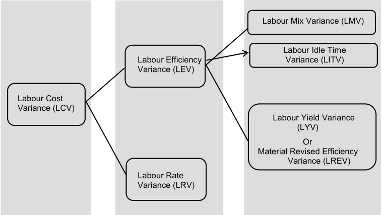
Labour Cost Variance (LCV)
Labour cost variance (also termed as direct wage variance) is the difference between the standard direct wages specified for the activity achieved and the actual direct wages paid. The formula for labour cost variance is:
LCV = (Standard Hours x Standard Rate) – (Actual Hours x Actual Rate)
OR
LCV = (SH x SR) – (AH x AR)
As the cost of labour is determined by labour time and wages, the labour cost variance is composed of either or both of variances relating to labour time and labour rate. As such, labour cost variance is analyzed into two separate variances, viz., wages (labour) rate variance and labour efficiency variance.
Labour Rate Variance
This is that portion of the wages variance which is due to the difference between the actual rate and standard rate of any specified. It is calculated like the materials price variance.
Labour Rate Variance = Actual Hours (Standard Rate – Actual Rate)
OR
LRV = AH x (SR – AR)
Causes of Wages (Labour) Rate Variance
Wage rate variance occurs due to the following causes:
- Change in basic wage structure or change in piece work rate.
- Overtime work in excess of that provided in the standard rate.
- Employment of one or more workers of a different grade than the standard grade.
- Payment of guaranteed wages to workers who are unable to earn their normal wages if such guaranteed wages form part of direct labour cost.
- New workers not being allowed full normal wage rates.
- Use of different method of payment i.e. payment of day rates while standards are based on piece work method of remuneration.
- Higher wages paid on account of overtime for urgent work.
- The composition of a gang as regards the skill and rate of wages being different from that laid down in the standard.
Wage rates are usually determined by factors beyond the control of the personnel department such as conditions in the labour market, wage awards by wage boards, etc. Wage rate variances are therefore, mostly uncontrollable except for the portion which arises due to deployment of wrong grade of labour for which the departmental executive may be held responsible.
Labour Time or Efficiency Variance
Also termed as labour efficiency variance, is that portion of the direct wages variance which is due to the difference between the standard labour hours specified and the actual labour hours expended. Obviously, this variance provides a key to the control of workers’ efficiency and labour cost. In effect, it is a usage variance. The computation of variance is as follows:
Labour Efficiency Variance = Standard Wage Rate (Standard Hours of Production – Actual Hours Worked)
OR
LEV = SR x (SH – AHW)
Causes of Labour Efficiency Variance
The causes giving rise to labour efficiency variance are as follows:
- Lack of proper supervision or stricter supervision than specified;
- Poor working conditions;
- Defective machinery and equipment;
- Discontentment in workers due to unsatisfactory personnel relations;
- Increase in labour turnover;
- Use of non-standard material requiring more or less operation time;
- Basic inefficiency of workers due to insufficient training, faulty instructions, incorrect scheduling of jobs, etc.
- Wrong selection of workers.
Labour Cost Variance = Labour Efficiency Variance + Labour Rate Variance
OR
LCV = LEV + LRV
Calculation of wage variance is illustrated below:
Example:
Assuming
Actual hours worked 5,600
Actual wage paid 7,840
Standard rate per hour 2
Standard hours produced 4,000
Answer:
Wages variance = Standard cost – Actual cost
(4,000 × 2) = 8,000 – 7,840 = 160 (F)
Wages rate variance = Actual hours (Standard rate – Actual rate)
= 5600 (2-1.4)
= 3,360 (F)
Actual Rate = 7840 = 1.4
5600
Labour efficiency rate variance
2 (4,000 – 5,600) = 3,200 (A)
Labour Cost Variance= Labour Rate Variance + Labour Efficiency Variance
= 3360 (F) + 3200 (A)
= 160 (F)
Labour efficiency variance is sub-divided into the following variances:
- Idle time variance
- Labour mix variance
- Labour yield variance (or Labour revised-efficiency variance)
Idle Time Variance
This variance which forms a portion of wages efficiency variance, is represented by the standard cost of the actual hours for which the workers remain idle due to abnormal circumstances.
Labour Idle Time Variance (LITV) =
(Actual hours paid for x Standard rate) – (Actual hours worked x Standard rate)
OR
Idle Hours x Standard rate.
It is always adverse. Suppose in the example given above the actual time includes 1,000 idle hours. The Idle Time Variance will then be 2,000 (A); the efficiency variance will be then 1,200 (A), making a total of 3,200 (A).
Labour Mix Variance
It is also known as Gang Composition Variance. This is a sub-variance which arises due to change in the composition of a standard gang or combination of labour force.
Labour mix variance =
(Actual hours at standard rate of actual gang – Actual hours at standard rate of standard gang)
OR
Standard rate (Revised standard labour hours – Actual labour hours)
OR
LMV = (RSH – AHW) x SR
Total actual time
Revised labour hours = Total standard time x Standard time
The calculation is just like that the materials. It is included in the efficiency or time variance discussed above.
Labour Yield Variance
This is due to the difference in the standard output specified and the actual output obtained. This is computed as follows:
Labour yield variance =
Standard labour cost unit (Actual output – Standard output)
OR
(Standard loss of actual total input – Actual loss) x Average standard rate per unit.
OR
LYV = SC p.u. (AY – SY)
Note: AY will never change. SY will calculate for actual mix of hour as under:
New SY = Old SY x TAH
TSH
If the actual output is more than standard output, it is favorable variance and vice versa.
