Materials Planning and Forecasting Techniques

The prime tool or technique of material planning is the Bill of Material Explosion, illustrated below:

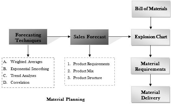
Materials Planning and Forecasting Techniques

Material planning is based on the demand planned for end products. Forecasting tools, such as weighted average method, time series method and exponential smoothening are some of the widely known methods used for material planning. Upon demand forecasting, the material planning activity is pursued. Bill of Materials is the document that details the requirement for a list of materials, unit consumption and code numbers for each product location. Explosion Chart is a chain of bills of materials clustered in a matrix, such that the combined requirements for varied components can be met. Materials requirement can be derived from demand forecast through explosion charts using bill of materials. Therefore, MRP leads to the development of delivery schedule of materials and hence, the purchase of those material requirements. It is an important part of forecasting techniques.

Moving Averages Method

A moving average is a technique to get an overall idea of the trends in a data set; it is an average of any subset of numbers. The moving average is extremely useful for forecasting long-term trends. You can calculate it for any period of time. For example, if you have sales data for a twenty-year period, you can calculate a five-year moving average, a four-year moving average, a three-year moving average and so on. Stock market analysts will often use a 50 or 200 day moving average to help them see trends in the stock market and (hopefully) forecast where the stocks are headed. It is an important part of forecasting techniques

Weighted Moving Average in Forecasting Techniques

When using an “average” we are applying the same importance (weight) to each value in the dataset. In the 4-month moving average, each month represented 25% of the moving average. When using demand history to project future demand (and especially future trend), it’s logical to come to the conclusion that you would like more recent history to have a greater impact on your forecast. We can adapt our moving-average calculation to apply various “weights” to each period to get our desired results. We express these weights as percentages, and the total of all weights for all periods must add up to 100%. Therefore, if we decide we want to apply 35% as the weight for the nearest period in our 4-month “weighted moving average”, we can subtract 35% from 100% to find we have 65% remaining to split over the other 3 periods. For example, we may end up with a weighting of 15%, 20%, 30%, and 35% respectively for the 4 months (15 + 20 + 30 + 35 = 100). It is an important part of forecasting techniques

Exponential Smoothing

This method is suitable for forecasting data with no trend or seasonal pattern. It does not display any clear trending behavior or any seasonality, although the mean of the data may be changing slowly over time.

Smoothing – Smoothing is a very common statistical process. In fact, we regularly encounter “smoothed” data in various forms in our day-to-day lives. Any time you use an average to describe something, you are using a smoothed number. If you think about why you use an average to describe something, you will quickly understand the concept of smoothing. For example, we just experienced the warmest winter on record. How are we able to quantify this? Well we start with datasets of the daily high and low temperatures for the period we call “Winter” for each year in recorded history. But that leaves us with a bunch of numbers that jump around quite a bit (it’s not like every day this winter was warmer than the corresponding days from all previous years). We need a number that removes all this “jumping around” from the data so we can more easily compare one winter to the next. Removing the “jumping around” in the data is called smoothing, and in this case we can just use a simple average to accomplish the smoothing. It is an important part of forecasting techniques

In demand forecasting, we use smoothing to remove random variation (noise) from our historical demand. This allows us to better identify demand patterns (primarily trend and seasonality) and demand levels that can be used to estimate future demand. The “noise” in demand is the same concept as the daily “jumping around” of the temperature data. Not surprisingly, the most common way people remove noise from demand history is to use a simple average—or more specifically, a moving average. A moving average just uses a predefined number of periods to calculate the average, and those periods move as time passes. For example, if I’m using a 4-month moving average, and today is May 1st, I’m using an average of demand that occurred in January, February, March, and April. On June 1st, I will be using demand from February, March, April, and May.

Exponential smoothing – If we go back to the concept of applying a weight to the most recent period (such as 35% in the previous example) and spreading the remaining weight (calculated by subtracting the most recent period weight of 35% from 100% to get 65%), we have the basic building blocks for our exponential smoothing calculation. The controlling input of the exponential smoothing calculation is known as the smoothing factor (also called the smoothing constant). It essentially represents the weighting applied to the most recent period’s demand. So, where we used 35% as the weighting for the most recent period in the weighted moving average calculation, we could also choose to use 35% as the smoothing factor in our exponential smoothing calculation to get a similar effect. The difference with the exponential smoothing calculation is that instead of us having to also figure out how much weight to apply to each previous period, the smoothing factor is used to automatically do that.

So here comes the “exponential” part. If we use 35% as the smoothing factor, the weighting of the most recent period’s demand will be 35%. The weighting of the next most recent period’s demand (the period before the most recent) will be 65% of 35% (65% comes from subtracting 35% from 100%). This equates to 22.75% weighting for that period if you do the math.

The next most recent period’s demand will be 65% of 65% of 35%, which equates to 14.79%. The period before that will be weighted as 65% of 65% of 65% of 35%, which equates to 9.61%, and so on. And this goes on back through all your previous periods all the way back to the beginning of time (or the point at which you started using exponential smoothing for that particular item).

You’re probably thinking that’s looking like a whole lot of math. But the beauty of the exponential smoothing calculation is that rather than having to recalculate against each previous period every time you get a new period’s demand, you simply use the output of the exponential smoothing calculation from the previous period to represent all previous periods.

The exponential smoothing calculation is as follows:

The most recent period’s demand multiplied by the smoothing factor.

PLUS

The most recent period’s forecast multiplied by (one minus the smoothing factor).

OR

(D*S)+(F*(1-S))

Where

• D = most recent period’s demand
• S = the smoothing factor represented in decimal form (so 35% would be represented as 0.35).
• F = the most recent period’s forecast (the output of the smoothing calculation from the previous period).

OR (assuming a smoothing factor of 0.35)

(D * 0.35) + ( F * 0.65)

Past Consumption Analysis

For continuously needed materials and the materials where no bill of materials is possible, this technique of analysis is adopted- The past consumption data is analyse and a projection for the future on the basis of past experience and future need is made. To prepare such a projection, “average” or “mean” consumption and the “standard deviation” are taken as bases and as guidelines for each item. It is an important part of forecasting techniques

Correlation

Correlation is a statistical technique that can show whether and how strongly pairs of variables are related. For example, height and weight are related; taller people tend to be heavier than shorter people. The relationship isn’t perfect. People of the same height vary in weight, and you can easily think of two people you know where the shorter one is heavier than the taller one. Nonetheless, the average weight of people 5’5” is less than the average weight of people 5’6”, and their average weight is less than that of people 5’7”, etc. Correlation can tell you just how much of the variation in peoples’ weights is related to their heights.

A positive correlation indicates the extent to which those variables increase or decrease in parallel; a negative correlation indicates the extent to which one variable increases as the other decreases.

A correlation coefficient is a statistical measure of the degree to which changes to the value of one variable predict change to the value of another. When the fluctuation of one variable reliably predicts a similar fluctuation in another variable, there’s often a tendency to think that means that the change in one causes the change in the other. However, correlation does not imply causation. There may be, for example, an unknown factor that influences both variables similarly.