A measure of spread, sometimes also called a measure of dispersion, is used to describe the variability in a sample or population. It is usually used in conjunction with a measure of central tendency, such as the mean or median, to provide an overall description of a set of data.
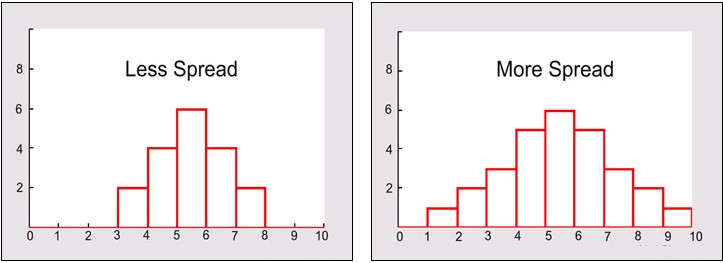
If the data is clustered around the center value, the “spread” is small. The further the distances of the data values from the center value, the greater the “spread”.
Measures of variability provide information about the degree to which individual scores are clustered about or deviate from the average value in a distribution.
Range
The simplest measure of variability to compute and understand is the range. The range is the difference between the highest and lowest score in a distribution. Although it is easy to compute, it is not often used as the sole measure of variability due to its instability. Because it is based solely on the most extreme scores in the distribution and does not fully reflect the pattern of variation.
Inter-quartile Range (IQR)
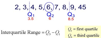
It divides the set into four equal parts (or quarters). The three values that form the four divisions are called quartiles: first quartile, Q1; second quartile (median), Q2, and third quartile, Q3. The interquartile range is the difference between the third quartile and the first quartile. You can think of the IQR (also called the midspread or middle fifty) as a “range” between the third and first quartiles. The IQR is considered a more stable statistic than the typical range of a data set, as seen in the first section. The IQR contains 50% of the data, eliminating the influence of outliers.
It provides a measure of the spread of the middle 50% of the scores. The IQR is defined as the 75th percentile – the 25th percentile. The interquartile range plays an important role in the graphical method known as the boxplot. The advantage of using the IQR is that it is easy to compute and extreme scores in the distribution have much less impact but its strength is also a weakness in that it suffers as a measure of variability.
Quartiles tell us about the spread of a data set by breaking the data set into quarters, just like the median breaks it in half.
Quartiles are a useful measure of spread because they are much less affected by outliers or a skewed data set than the equivalent measures of mean and standard deviation. The interquartile range describes the difference between the third quartile (Q3) and the first quartile (Q1), telling us about the range of the middle half of the scores in the distribution. Hence, for our 100 students:
Interquartile range = Q3 – Q1
= 71 – 45
= 26
Variance (s2)
The variance is a measure based on the deviations of individual scores from the mean. As, simply summing the deviations will result in a value of 0 hence, the variance is based on squared deviations of scores about the mean. The sum of the squared deviations, is divided by N (population) or by N – 1 (sample). The result is the average of the sum of the squared deviations and it is called the variance. The variance is not only a high number but it is also difficult to interpret because it is the square of a value.
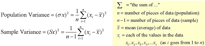
The variance achieves positive values by squaring each of the deviations instead. Adding up these squared deviations gives us the sum of squares, which we can then divide by the total number of scores in our group of data.
Process
- Find the mean (average) of the set.
- Subtract each data value from the mean to find its distance from the mean.
- Square all distances.
- Add all the squares of the distances. Divide by the number of pieces of data (for population variance).
Standard deviation (s)
The standard deviation is defined as the positive square root of the variance and is a measure of variability expressed in the same units as the data. The standard deviation is very much like a mean or an “average” of these deviations.
The standard deviation is a measure of the spread of scores within a set of data. Usually, we are interested in the standard deviation of a population. However, as we are often presented with data from a sample only, we can estimate the population standard deviation from a sample standard deviation. These two standard deviations – sample and population standard deviations – are calculated differently. In statistics, we are usually presented with having to calculate sample standard deviations.
Sample
Discrete Distribution Question – The weights of 5 ear-heads of sorghum are 100, 102,118,124,126 gms. Find the standard deviation.
Solution
| x | x2 |
| 100 | 10000 |
| 102 | 10404 |
| 118 | 13924 |
| 124 | 15376 |
| 126 | 15876 |
| 570 | 65580 |
Standard Deviation = 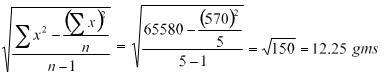
Continuous Distribution Question – The Frequency distributions of seed yield of 50 sesame plants are given below. Find the standard deviation.
| Seed yield in gms (x) | 2.5-35 | 3.5-4.5 | 4.5-5.5 | 5.5-6.5 | 6.5-7.5 |
| No. of plants (f) | 4 | 6 | 15 | 15 | 10 |
Solution
| Seed yield in gms (x) | No. of Plants f | Mid x | d= (x-A)/c | df | d2 f |
| 2.5-3.5 | 4 | 3 | -2 | -8 | 16 |
| 3.5-4.5 | 6 | 4 | -1 | -6 | 6 |
| 4.5-5.5 | 15 | 5 | 0 | 0 | 0 |
| 5.5-6.5 | 15 | 6 | 1 | 15 | 15 |
| 6.5-7.5 | 10 | 7 | 2 | 20 | 40 |
| Total | 50 | 25 | 0 | 21 | 77 |
A=Assumed mean = 5
n=50, C=1
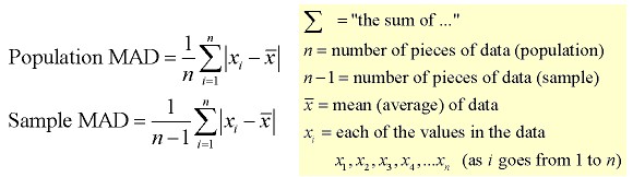
Mean Absolute Deviation (MAD)
The mean absolute deviation is the average (mean) of the absolute value of the differences between each piece of data in the data set and the mean of the set. It measures the average distances between each data element and the mean.
Process
- Find the mean (average) of the set.
- Subtract each data value from the mean to find its distance from the mean.
- Turn all distances to positive values (take the absolute value).
- Add all of the distances. Divide by the number of pieces of data (for population MAD).
It is the mean of the distances of each value from their mean. It is a robust measure of the variability of a univariate sample of quantitative data. It can also refer to the population parameter that is estimated by the MAD calculated from a sample.
Consider the data (1, 1, 2, 2, 4, 6, 9). It has a median value of 2. The absolute deviations about 2 are (1, 1, 0, 0, 2, 4, 7) which in turn have a median value of 1 (because the sorted absolute deviations are (0, 0, 1, 1, 2, 4, 7)). So the median absolute deviation for this data is 1.
Coefficient of variation (cv)
Measures of variability cannot be compared like the standard deviation of the production of bolts to the availability of parts. If the standard deviation for bolt production is 5 and for availability of parts is 7 for a given time frame, it cannot be concluded that the standard deviation of the availability of parts is greater than that of the production of bolts thus, variability is greater with the parts. Hence, a relative measure called the coefficient of variation is used. The coefficient of variation is the ratio of the standard deviation to the mean. It is cv = σ / µ for a population and cv = s/ or Standard Deviation / Mean * 100, for a sample.
Sample
Consider the measurement on yield and plant height of a paddy variety. The mean and standard deviation for yield are 50 kg and 10 kg respectively. The mean and standard deviation for plant height are 55 am and 5 cm respectively.
Here the measurements for yield and plant height are in different units. Hence the variabilities can be compared only by using coefficient of variation.
For yield, CV= 10/50 * 100 = 20%
For plant height, CV= 5/55 * 100 = 9.1%
The yield is subject to more variation than the plant height.
