This section coves advanced topics in inventory and warehouse analytics.
Lot size refers to the quantity of an item ordered for delivery on a specific date or manufactured in a single production run. In other words, lot size basically refers to the total quantity of a product ordered for manufacturing. In financial markets, lot size is a measure or quantity increment suitable to or précised by the party which is offering to buy or sell it. A simple example of lot size is: when we buy a pack of six chocolates, it refers to buying a single lot of chocolate.
Inventory Models
There are several ways of classifying the inventory models. Some attributes, useful in distinguishing between various inventory models are
Number of Items
- Single Item – This type of model recognizes one type of product at a time. If the demand
- rate changes from period to period, then the problem becomes that of a dynamic lot-sizing problem.
- Multi Item – This type of mode1 considers a number of products simultaneously. These products musr have at least one interrelating or binding factor such as budget or capacity constraint or a common setup.
Stocking Points
- Single Echelon Models – Only one stocking location is considered.
- Multi Echelon Models – More than one interconnected stocking locations are considered.
Frequency of Review
This is the frequency of assessment of the current stock position of the system and the implementation of the ordering decision.
- Periodic – Placement of orders is done at discrete points in time, with a given periodicity.
- Continuous – Order placement can occur at any time.
Order Quantity
- Fixed – Order quantity is fixed to the same amount each time.
- Variable – Order quantity can be variable.
Planning Horizon
- Finite – Demands are recognized over a limited number of periods.
- Infinite – Demands are recognized over an unlimited number of periods.
Demand
- Deterministic – Demands are known with certainty over the planning horizon.
Lead Trine
- Zero – No time elapses between placement and receipt of orders.
- Non Zero – Significant time elapses between the placement and receipt of orders. This
- time may be constant or random.
Capacity
- Capacitated – There are capacity restrictions on the amount produced or ordered.
- Un-capacitated – Capacity is assumed to be unlimited.
Unsatisfied Demand
- Not allowed – In this case. a11 demand is met and no shortages are allowed.
- Allowed – Demand not satisfied in a particular period may be retained and satisfied in a
- future period (backlogging). partially retained and partially lost or completely lost (no backlogging).
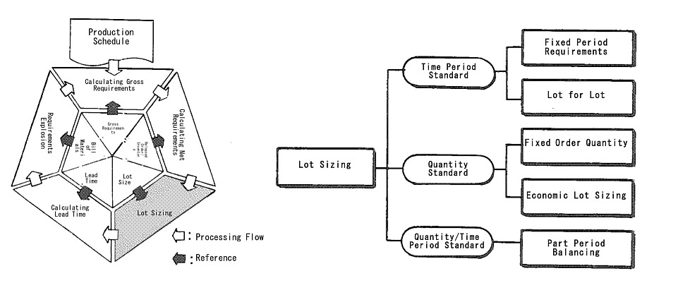
Lot Sizing
Lot sizing is to unify the calculated net requirements by a certain unit considering cost reduction and work efficiency.
There are two main types of lot sizing: a method to unify in terms of the period and another method to unify in terms of the quantity. The former includes “Fixed Period Requirements”, which, generally speaking, is suitable for the relatively expensive items whose demand occurs irregularly. The latter includes “Fixed Period Requirements” or “Economic Lot Sizing”, which is suitable for items whose demand is relatively stable. In addition to these types, there are any other types of lot sizing as shown in the figure.
Lot Sizing Techniques
- Lot for Lot (LFL): Order the exact amount of the net requirement each period. A lot-sizing technique that generates planned orders in quantities equal to the net requirements in each period. In MRP logic, planned order releases are equal to net requirements for LFL lot sizing rule.
- Fixed Order Quantity (FOQ): A lot-sizing technique that will always cause planned or actual orders to be generated for a predetermined fixed quantity, or multiples, if net requirements for the period exceed the fixed order quantity. The order quantity is decided arbitrarily.
- Single Lot: Order quantity is equal to the total requirement and only one order is to be placed.
- Economic Order Quantity (EOQ): Order an EOQ or ERL amount. This is a fixed order quantity rule with order quantity equal to EOQ.
- Least Unit Cost (LUC): Order the net requirement for the current period or current plus next or current plus next two and so on, depending upon which gives the lowest unit cost. A dynamic lot-sizing technique that chooses the lot size with the lowest unit cost by adding ordering cost and inventory carrying cost for each trial lot size and dividing by the number of units in lot size. The unit cost is calculated from the period next to a period with a planned order receipt, until the lowest unit is found.
- Least Total Cost (LTC): A dynamic lot-sizing technique that calculates the order quantity by comparing the setup (or ordering) cost and the carrying cost for various lot sizes, and selects the lot where these costs are most nearly equal. Least total cost occurs where the accumulated carrying cost equals a setup cost.
- Minimum Cost Period (MCP): Order quantity is selected in such a way the cost period must be minimum.
- Part-Period Algorithm (PPA): Use the ratio of ordering and carrying costs to derive a part-period number and use the number as a criterion for cumulating requirements.
- Part Period Balancing (PPB): One part-period of an item means one unit of that item is carried in inventory for one period. Economic part-period (EPP) is the quantity of an item which, if carried in inventory for one period, would result in a carrying cost equal to setup cost. Therefore, EPP = Ordering Cost / Unit Carrying Cost. PPB is a dynamic lot-sizing technique that uses the same logic as LTC method.
- Period Order Quantity (POQ): Divide the Economic Order Quantity (EOQ) into the annual demand and order that many times per year.
- Periodic Review System (PRS): A periodic reordering system where the time interval between orders is fixed, but the size of the order is variable. An order is placed every n time periods. The time interval is determined arbitrarily. This approach as well as the next approach (POQ) is also known as fixed reorder cycle inventory models.
| Lot Sizing | Lot Size | Order Interval |
| FOQ, EOQ | Fixed | Variable |
| PRS, POQ | Variable | Fixed |
| LUC, LTC, PPB | Variable | Variable |
Cushions
The environment of operations planning and control is uncertain. The best way to solve the uncertainty problem is to eliminate the uncertainty, i.e., to make the environment more stable through the efforts such as increasing the similarity of product and process design, shortening the setup time, decreasing the lot sizes, decreasing the manufacturing lead-times, smoothing the supply channels, etc.
Safety Stock – The safety stock is used to cover the random uncertainties caused by unknown factors. When the source of an uncertainty is known, such as suppliers’ late delivery, approaches other than safety stock should be used to resolve it. Masking the source of the problem causing an uncertainty with safety stock will prevent the actual cause of the problem from being addressed.
Safety Time – If a supplier’s delivery tends to be late, increasing the lead-time will not be an effective method of smoothing production. Suppliers tend to ignore orders with long lead-times in favor of urgent orders placed by other buyers.
Safety Capacity – In priority planning, sometimes scheduled quantities require available capacity that exceeds current productive capacity. Safety capacity provides protection from planned activities, such as resource contention and preventive maintenance, and unplanned activities, such as additional requirement, resource breakdown, poor quality, rework, or lateness.
Lot-size Inventory
In order to take advantage of quantity price discounts, reduce shipping and setup costs, or address similar considerations, items are manufactured or purchased in quantities greater than needed immediately. Since it is more economical to produce or purchase less frequently and in larger quantity, inventory is established to cover needs in periods when items are not replenished.
Inventory Costs related to Lot Sizing
Ordering Cost – Ordering costs are the costs associated with placing an order with the factory or a supplier. The ordering cost does not depend on the quantity ordered. It is a composite of all costs related to placing purchase orders or preparing shop orders, including
- Paperwork,
- Work station setups,
- Inspection, scrap, and rework associated with setups,
- Record keeping for work-in-process.
Carrying Cost – Carrying cost is the total of costs related to maintaining the inventory, including
- Capital cost invested in inventory, or foregone earnings of alternate investment,
- Storage costs for space, equipment, and people,
- Taxes and insurance on inventory,
- Obsolescence caused by market, design, or competitors’ product changes,
- Deterioration from long-term storage and handling,
- Record keeping for inventory.
Factors affecting Lot Sizing Decision
Several parameters affect lot sizing and should be considered. They are listed below.
- Degree of information – Does parameter have a fixed known value. Stochastic models contain parameters which are random variables.
- Time scale – Planning may be done in small (hours, shifts or days), or large (weeks, months) discrete periods or over continuous time scale. One of the ancestors of the continuous time models is the Economic Order Quantity (EOQ) model, which is a continuous time model with an infinite time horizon.
- Horizon – The planning horizon may be assumed to be infinite, finite, or variable. Generally, discrete time problems consider finite horizon while continuous time problems are based on infinite time horizon. A medium-range (short-range) finite planning horizon problem has a time horizon that is typically months (weeks) away.
- Number of items – If there is no (relevant) interdependency between items, either because of joint utilization of capacity or parent-component relationship, independent single-item problems occur.
- Number of levels – If there is no parent-component relationship between items a single-level problem arises, and otherwise we have a multi-level problem. The parent-component relationships are defined by the item structure. Some of the well-known product structures are serial, assembly (in-tree), and general. Also, the term stage is sometimes used instead of level.
- Relevant costs – In addition to unit production cost, these include:
- Setup related costs: These are the costs incurred each time a setup takes place for an item on a facility. If the setup costs depend on the sequence in which the items are scheduled a problem with sequence dependent setup costs arises.
- Inventory related costs: These include holding costs which are the costs incurred for holding an item in inventory during one or more periods, and consist mainly of the costs of capital tied up in inventory, potential spoilage or obsolescence, taxes, insurance and warehouse operation costs.
- Capacity related costs: These are costs incurred for using regular capacity and/or extra capacity (overtime costs, cost due to subcontracting or changing the workforce level).
- Resource constraints – Disregarding resource constraints to an incapacitated problem, otherwise to a capacitated one. A single resource constraint in the multi-level case is often called a “bottleneck”. If more than one machine is considered a multi-machine problem arises, otherwise a single-machine problem.
- Objectives – Usually, the total costs have to be minimized. Further possible objectives can be maximization of the service level or smoothing the production load.
Lot Size Inventory Problem
Two basic questions to be answered in most of the inventory situations are:
- when to order (the reorder point)
- how much to order (the lot size).
When the demand rate is constant over time. the associated problem of planning is rather simple because the use of the Classical Economic Order Quantity Model (EOQ Model) gives us optimal results. But when the demand rate varies over time i.e. not necessarily constant from one period to another, the associated problem of planning is a bit more challenging and is said to be dynamic in nature.
Solution Approaches
A dynamic programming algorithm was suggested to deal with the uncapacitated inventory control problem. Though the approach gives optimal results, the complex nature of dynamic programming makes it difficult to understand and therefore makes it practically useless. There are numerous heuristic methods available which are easy to use but not necessarily optimal.
In certain practical situations such as for dedicated production lines. group technology and FMS. It is impossible to ignore setup costs or setup times. Each time a setup is done. a cost is incurred. This suggests an integer linear programming approach with some binary variables representing the setups. The main underlying assumption in most of the models is that “demand is deteministically known”. But demand is always forecasted. and most of the times the forecasts do not turn out to be precisely correct.
Linear Programming – It is a mathematical method of allocating scarce resources to achieve an objective, such as maximizing profit. Linear programming involves the description of a real-world decision situation as a mathematical model that consists of a linear objective function and linear resource constraints. Once the problem has been identified. the goals of management established. and the applicability of the linear programming determined. The next step in solving an unstructured, real world problem is the formulation of a mathematical model. This entails three major steps:
- Identification of solution variables (the quantity of the activity in question).
- The development of an objective function that is a linear relationship of the solution variables, and
- The determination of system constraints, which are also linear relationships of the decision variables, which reflect the limited resources of the problem.
In each problem decision variables denote a level of activity or quantity produced. The objective function represents the sum total of the contribution of each decision variable in the model towards an objective. The constraints of a linear programming model represent the limited availability of resources in the problem.
Fuzzy Set Theory – Theory of fuzzy sets is basically a theory of graded concepts. A central concept of fuzzy set theory is that it is permissible for an element to belong partly to a fuzzy set.
Goal Programming – Any goal-programming model will be formulated by using two types of variables
- decision variables (the x’s) and the
- deviational variables (the d’s and d-s).
Two classes of constraints can exist in a given goal programming model i.e. structural constraints., which are generally considered
- environmental constraints and are not directly related to goals
- goal constraints which are directly related to goals.
Finally, while in most cases a goal constraint will contain both an underachievement (d-) and an over achievement (d’) devistional variable, even when both do not appear in the objective function. it is not mandatory that both be included. Omission of either type of deviational variable in the goal constraint, however, bounds the goal in the direction of omission. That is. omission of d’ places an upper bound in the goal. while omission of d- forces a lower bound on the goal.
It is important to decide the priorities for the goals. First of all. the goal with the highest priority is exclusively considered in the objective function and the problem is solved minimizing the deviation of this goal.
Lot Size Optimization
Best-of-breed lot sizing approaches allow the following
- Include both supply and demand variability
- As a required step, conduct capacity analysis of the process
- Analyze entire product mix concurrently
- Require minimal special-expertise
- Present results in an easy-to-visualize format
- Use data already in ERP when at all possible
- As an option: Include analysis of stocking levels as well
Real World Lot Sizing in SAP
The Lot sizing procedures in SAP are categorized as static lot sizing procedures, periodic lot sizing procedures and optimum lot sizing procedures. The most famous lot sizing procedures are the static lot sizing procedures and periodic lot sizing procedures.
Static Lot Sizing Procedures
The static lot sizing procedures are namely – the ‘exact lot sizing’, fixed lot sizing and ‘replenish to maximum stock level’.
When the lot size is “EX” or exact lot size, the system creates planned orders or procurement proposals to cover the exact shortage requirement. The lot size is the whole shortage quantity required to satisfy the demand. That is, if the requirement is for a quantity of 112 units, the proposal will be created for an exact 112 units.
On the other hand if the lot sizing procedure is “fixed lot size”, then the total requirement quantity as proposed by the system, to cover the shortages is divided in to the number of fixed quantities as included in the material master (MRP 1 view), for example, if the lot size is fixed as 100 Units and the shortage quantity is 500, then the system will create 5 planned orders to cover the shortages.
Similarly if the lot size of the material is “replenish to maximum stock level” (Lot Size – “HB” for example oil tankers or barges) then on shortages of the requirement quantities the system creates planned orders to fill it to the maximum stock level.
