Various quantitative models are used to help determine the best locations of facilities. There are some widely known general models that can be adapted to the needs of variety of systems. These are explained below:
Simple Median Model
Suppose we want to locate a new plant that will receive shipments of raw materials from two sources: F1 and F2. The plant will create finished goods that must be shipped to two distribution warehouses F3 and F4 Given these four facilities, where should we locate the new plant to minimize annual transportation cost for the network of facilities?
The median model can help answer this question. The model considers the volume offloads transported on rectangular paths. All movements are made in east-west or North-south directions; diagonal moves are not considered. The simple median model provides an optimal solution.
Table 5.2 shows the number of loads Li to be shipped annually between each existing facility F, and the new plant; it also shows the coordinate location’ (Xi, Yi) of each existing facility Fi and the cost Ci to move a load one distance unit to or from Fi. We let Di be the distance units between facility Fi and the new plant. The total transit cost, then, is the sum of the products CiLiDi for all i: cost times loads times distance.
n
Total transportation cost = ∑ CiLiDi Equation 5.1 i=1
Table 5.2 Locations of existing facilities and number of loads to be moved
Coordinate Location (Xi, Yi) of Fi
| Existing Facility Fi | Annual Loads Li between Fi and New Plant | Cost Ci to move one Load One distance Unit | (Xin Yi |
| F1 | 755 | 1 | (20, 30) |
| F2 | 900 | 1 | (10, 40) |
| F3 | 450 | 1 | (30, 50) |
| F4 | 500 | 1 | (40, 60) |
| Total | 2,605 |
Since all loads must be on rectangular paths, distance between each existing facility and the new plant will be measured by the difference in the x-coordinates and the difference in the y- coordinates (see figure 5.1). If we let (x0, y0) be the coordinates of a proposed new plant, then
Di = |xi – x0| + |yi- y0|
Our goal is to find values for x0 and y0 (new plant) that result in minimum transportation costs. We follow three steps:
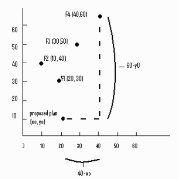
Figure 5.1: Sources of raw materials and distribution warehouses
- Identify the median value of the loads Li moved.
- Find the x-coordinate of the existing facility that sends (or receives) the median load.
- Find the y-coordinate value of the existing facility that sends (or receives) the median load.
The x- and y- coordinates found in steps 2 and 3 define the new plants best location.
Application of the Model: Let us apply the three steps to the data in Table 5.1.
- Identify the median load: The total number of loads moved to and from the new plant will be 2,605. If we think of each load individually and number them from 1 to 2,605, then the median load number is the “middle” number – that is, the number for which the same number of loads fall above and below. For 2,605 loads, the median load number is 1,303, since 1302 loads fall above and below load number 1,303. If the total number of loads were even, we would consider both “middle” numbers.
- Find the x-coordinate of the median load: First we consider movement of loads in the x-direction. Beginning at the origin the figure 5.1 and moving to the right along the x-axis, observe the number of loads moved to or from existing facilities. Loads 1- 900 are shipped by F2 from location x = 10. Loads 901-1,655 are shipped by F1 from location x =20. Since the median load falls in the interval 901-1,655, x = 20 is the desired x-coordinate location for the new plant.
- Find y-coordinate of the median load: Now consider the y-direction of load movements. Begin at the origin of Figure 5.1 and move upward along the y-axis. Movements in the y direction begin with loads 1-755 being shipped by F1 from location y=30. Loads 756-1,655 are shipped by F2 from location y=40. Since the median load falls, in the interval 756-1655, y=40 is the desired y-coordinate for the new plant.
The optimal plant location, x =20 and y=40, results in minimizing annual transportation costs for this network of facilities. To calculate the resulting cost, we use equation 5.1:
n
Total transportation cost = ∑ CiLi (x| xi| + |y-yi|) i=1
Total cost, $45,550
Some concluding remarks are in order: First, we considered the case in which only one new facility is to be added. Second, you should not an important assumption of this model: Any point in the x-y coordinate system is an eligible point for locating the new facility. The model does not consider road availability, physical terrain, population densities, or any other of the many important location considerations. The task of blending model results with other major considerations to arrive at a reasonable location choice is a major managerial responsibility.
Linear Programming: Linear programming may be helpful after the initial screening phase has narrowed the feasible alternative sites. The remaining candidates can then be evaluated. , one at a time, to determine how well each would fit in with existing facilities, and alternatives that leads the best overall system( network) performance can be identified. Most often, overall transportation cost is the criterion used for performance evaluation. A special type of linear programming called the distribution or transportation method is particularly useful in location planning. The mechanics of this technique are omitted in the example.
Example: Alpha Processing Company has three Midwestern production plants located at Evansville, Indiana: Lexington, Kentucky; and Fort Wayne, Indiana. Five-year operations plans require that 200 shipments of raw materials be delivered annually to the Evansville plant, 300 shipments to Lexington, and 400 shipments to Fort Wayne. Currently, Alpha has two sources of raw materials, one at Chicago, Illinois, the other at Louisville, Kentuchy. The Chicago source can supply 300 shipments per year and Louisville, 400. An additional source of raw materials must therefore be found. Preliminary screening by Alpha has narrowed the choice to two attractive alternatives: Columbus, Ohio and St. Louis, Missouri. Each of these sites can supply 200 shipments per year. Alpha has decided to make its selection on the basis of minimizing transportation costs. Estimates of the cost per shipment from each source to each plant are shown in Table 5.3
The cost analysis for Alpha Company proceeds in two stages.
- The first stage determines the number of shipments from each source to each plant that yields the lowest possible cost, assuming Columbus is the third source.
- The second stage determines the number of shipments yielding the lowest possible cost, assuming St. Louis is the third source. The minimum Columbus cost is compared to the minimum St. Louis cost, and the cheaper site is selected. A final solution for Alpha is shown in Figure 5.2
Table 5.3 Sources, destinations, and costs of raw material shipments
| Destination (cost per shipment) | ||||
| Source | Evansville | Lexington | Fort Wayne | Shipments Available |
| Chicago | $200 | $200 | $200 | 300 |
| Louisville | 100 | 100 | 300 | 400 |
| Columbus | 300 | 200 | 100 | 200 |
| St. Lousis | 100 | 300 | 400 | 200 |
| Shipments needed | 200 | 300 | 400 |
If Columbus is selected, minimum annual shipping costs will be $120,000. This occurs if 100 shipments go from Chicago to Evansville (costing $200 each), 200 shipments from Chicago to Fort Wayne (costing $200 each), 100 from Louisville to Evansville ($100 each), 300 from Louisville to Lexington ($100 each), and 200 from Columbus to Fort Wayne ($100 each). These shipment quantities, shown beneath the diagonal lines in part (a) of Figure 5.2, satisfy the raw material needs of all three plants and fully uses the capacities of all three raw materials sources. Any other pattern of shipments will result in higher annual shipping costs.
Part (b) of Figure 5.2 shows that if St. Louis is selected he minimum annuals cost will be $140,000. Columbus is therefore selected, at a cost of $120,000 annually.
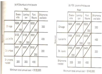
Figure 5.2 Evaluation of Alpha transportation costs
Notice that the linear programming model differs from the simple median model in two fundamental ways
- Number of alternative sites: The simple median model assumes that all locations are eligible to be the new location. The linear programming model, in contrast, considers only a few locations pre-selected from preliminary feasibility studies.
- Direction of transportation movements: The simple median model assumes that all shipments move in rectangular patterns. The linear programming model does not so assume.
Behavioral Impact in Facility Location: Our previous discussions of models focused on the cost consequences. But costs are not the whole story, and models can’t account for aspects of a problem that are not quantifiable. New locations require that organizations establish relationships with new environments and employees, and adding or deleting facilities requires adjustments in the overall management system. The organization structure and modes of making operating decisions must be modified to accommodate the change. These hidden “system costs” are usually excluded from quantitative models, and yet they are very real aspects to location decisions.
Cultural Differences: The decision to locate a new facility usually means that employees will be hired from within the new locate. It also means that the organization must establish appropriate community relations to “fit into” the locale as a good neighbor and citizen. The organization must recognize the differences in the way people in various ethnic, urban, suburban, and rural communities react to new businesses. Managerial style and organizational structure must adapt to the norms and customs to local subcultures. Employees’ acceptance of authority may vary with subcultures, as do their life goals, beliefs about the role of work, career aspirations, and perceptions of opportunity. These cultural variations in attitude impact on the job behavior and talent.
At the international level are even greater cultural differences. Compare, for example, the Japanese work tradition with that of Western industrial society. Japanese workers are often guaranteed lifetime employment. Management decisions usually are group rather than individual decisions. Employee compensation is determined by length of service, number of dependents, and numerous factors apart from the employee’s productivity. Obviously operations managers in Japan face a very different set of managerial problems from their U.S. counterparts. Wage determination, employee turnover, hiring and promotion practices are not at all the same.
The European social system, as another example, has resulted in a more “managerial elite” in their organizations than in U.S. organizations. Because of education, training and socialization, including a lifelong exposure to a relatively rigid class system; lower subordinates are not prepared to accept participative managerial styles. This has resulted in organizations more authoritarian/centralized than participative /decentralized.
Locating a new facility in a new culture is not simply a matter of duplicating a highly refined manufacturing process. Merely transferring tools and equipment is not adequate. Managerial techniques and skills, in proper mixture, must be borrowed from the culture, and so must the cultural assumptions that are needed to make them work. Clearly, the economic, political makeup of a society has far-reaching effects on the technological and economic success of multinational location decisions.
Job Satisfaction: In recent years managers have been very concerned about employee job satisfaction because it affects how well the organization operates. Although no consistent overall relationship between job satisfaction and productivity seems to exist, other consistent relationships have been found. As compared with employees with low job satisfaction, those expressing high job satisfaction exhibit the following characteristics.
- Fewer labor turnovers
- Less absenteeism
- Less tardiness
- Fewer grievances
These four factors can substantially affect both costs and disruptions of operations. But how is job satisfaction related to facility location? There is some evidence that satisfaction is related to community characteristics such as community prosperity, small town versus large metropolitan locations, and the degree of unionization. Accordingly, a company with facilities in multiple locations can expect variations in employees’ satisfaction due to variations in attitudes and value systems across locations.
