
Linear programming (LP; also called linear optimization) is a method to achieve the best outcome (such as maximum profit or lowest cost) in a mathematical model whose requirements are represented by linear relationships. Linear programming is a special case of mathematical programming (mathematical optimization).
More formally, linear programming is a technique for the optimization of a linear objective function, subject to linear equality and linear inequality constraints. It’s feasible region is a convex polyhedron, which is a set defined as the intersection of finitely many half spaces, each of which is defined by a linear inequality. Its objective function is a real-valued affine function defined on this polyhedron. A linear programming algorithm finds a point in the polyhedron where this function has the smallest (or largest) value if such a point exists.
Standard form is the usual and most intuitive form of describing a linear programming problem. It consists of the following three parts:
- A linear function to be maximized g.
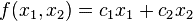
- Problem constraints of the following form e.g.
- Non-negative variables g.

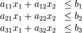
The problem is usually expressed in matrix form, and then becomes

Other forms, such as minimization problems, problems with constraints on alternative forms, as well as problems involving negative variables can always be rewritten into an equivalent problem in standard form.
The transformation of a linear program to one in standard form may be accomplished as follows. First, for each variable with a lower bound other than 0, a new variable is introduced representing the difference between the variable and bound. The original variable can then be eliminated by substitution. For example, given the constraint

a new variable, y1, is introduced with

The second equation may be used to eliminate x1 from the linear program. In this way, all lower bound constraints may be changed to non-negativity restrictions. Second, for each remaining inequality constraint, a new variable, called a slack variable, is introduced to change the constraint to an equality constraint. This variable represents the difference between the two sides of the inequality and is assumed to be nonnegative. For example the inequalities
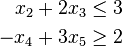
are replaced with
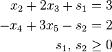
It is much easier to perform algebraic manipulation on inequalities in this form. In inequalities where ≥ appears such as the second one, some authors refer to the variable introduced as a surplus variable. Third, each unrestricted variable is eliminated from the linear program. This can be done in two ways, one is by solving for the variable in one of the equations in which it appears and then eliminating the variable by substitution. The other is to replace the variable with the difference of two restricted variables. For example if z1 is unrestricted then write
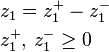
The equation may be used to eliminate z1 from the linear program. When this process is complete the feasible region will be in the form

It is also useful to assume that the rank of A is the number of rows. This results in no loss of generality since otherwise either the system Ax >= b has redundant equations which can be dropped, or the system is inconsistent and the linear program has no solution.
Sample Problem
A firm produces products A, B & C each of which passes through three departments Fabrication, Finishing & Packaging. Each unit of product A requires 3, 4 & 2, a unit of product B requires 5, 4 & 4 while each unit of C requires 2, 4 & 5 hours respectively in the three departments. Everyday 60 hours are available in Fabrication, 72 hours are available in Finishing and 100 hours in Packaging department. If the unit contribution of product A is Rs.5/-, product B is Rs.10/-, product C is Rs.8/-, determine the number of units of each of the products, that should be made each day to maximize the total contribution.
Solution
Given Case is analyzed as per guidelines and following facts are established, as
- This is a case of profit maximization. An optimal solution maximizing profits is contemplated.
- Company is considering producing products A, B & C.
- Expected profit contribution by a unit of A is Rs.5/-, by a unit of B is Rs.10/-and by a unit of C is Rs. 8/-h. Resource requirements of each product in units, decision variables and resources availability in appropriate units are tabulated as
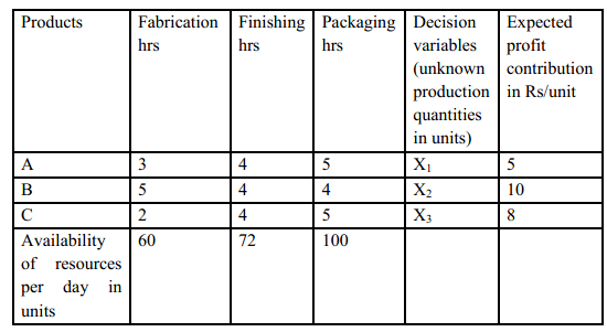
Let unknown quantity X1 units of A, unknown quantity X2 units of B and an unknown quantity X3 units of C be produced. The model will finally give the values of decision variables X1, X2 & X3 for maximum profit at optimum level. Contribution per unit for A, B & C are Rs 5/-, Rs 10/- & Rs 8/-. Unknown production quantities X1, X2 and X3 are decision variables. The objective function for case is written as below.
5X1 + 10X2 +8X3 = Z (Z is the total profit per day) which is to be maximized
The constraint relationships are
3X1+ 4X2+5X3 <=60 (1) Fabrication Constraint
5X1+ 4X2+4X3<=72 (2)Finishing Constraint
2X1+ 4X2+5X3<=100 (3)Packaging Constraint
X1, X2, X3 ≥0 Non negativity constraint
The mathematical formulation suitable for simplex method is written in terms of decision variables, slack variables and their coefficients. While X1, X2, X3 are decision variables S1,S2& S3 are slack variables introduced to establish equality between LHS & RHS. The objective function is
5X1+ 10X2+8X3+0S1 +0S2+0S3 = Z (Z is the total profit per day) which is to be maximized.
Now Constraints are
3X1+ 4X2+5X3+S1+0S2+0S3 = 60 (1) Fabrication Constraint
5X1+ 4X2+4X3+ 0S1+S2+0S3= 72 (2)Finishing Constraint
2X1+ 4X2+5X3+ 0S1+0S2+S3= 100 (3)Packaging Constraint
X1,X2, X3, S1, S2, S3≥0 Non negativity constraint
From the above standard form, a feasible starting solution is written as follows. Putting X1= 0, X2= 0, X3= 0, Hence, S1= 60, S2=72,S3=100
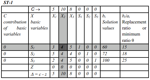
From the information collected, following simplex table ST-1 is constructed as
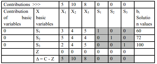
The identity matrix can be seen as marked by the shaded area. The variables forming the identity matrix are put in the basis.
- Calculation of Z row values – Calculations for the Z value for column of X1 is as
- Coefficient of X1in the first row of S1=3
- Contribution of basic variable in first row,S1=0
- Product of the above two values in first row is 0
- Similarly the products for second and third rows are also 0
- Hence Z value for first column is 0
- Z values for other variables are similarly calculated
The table shows that the index row (Net Evaluation Row or NER) values are not non-positive. Hence the conclusion is that the solution is not optimal but needs further improvement. The table below shows key column, key row, and key element, information required to perform iteration and move towards optimality.
Using the key information from the solution in ST1, the solution is further improved and written in ST2. The calculations for a new cell value are shown below.
New value for a cell (S2-X1) in a particular row rj (row of S2) = value in the same cell of previous table (5) –value in the intersection of key column and the particular row rj in previous table (4) X value in the corresponding cell in the row where basic variable has been changed in the new table (3/4). New value for (S2-X1) = [5–4 X (3/4)] = 2
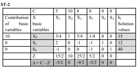
It is found that all NER values are non-positive hence the conclusion is that the solution now is optimal.