File Management

Creating a workbook

Workbook can be created in various ways like creating a new blank document or creating a workbook from a copy of an existing workbook by using the task pane. Click File, point to New option and click. A new blank file is opened. The other way to open a new file is to press “CTRL” key and then press “N” holding down the CTRL key and this key press sequence is denoted as “CTRL + N”.

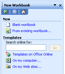
New workbook

Saving a workbook

To save active workbook to a file on our hard disk,   press “Control” and “S” key or in File Menu click on save option (from the menu bar). Saving first time for new document opens “Save As” dialog box but after first time save, no dialog box opens on consecutive saves.

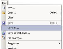
Save As in File Menu

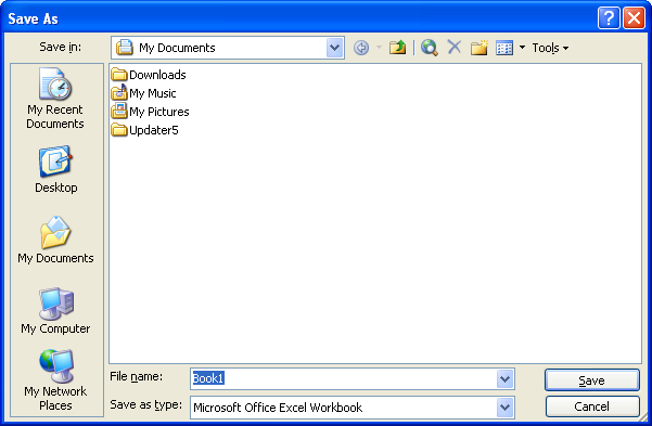
Save As dialog box

The Save As dialog box specifies the location to save the file and its file name. The “Save in” drop down list displays the default folder as the location where the file will be saved. File Name text box displays the proposed file name. The file list box displays the names of any word documents in the default location. The windows documents can have up to 256 characters in the file name. Names can contain letters or numerals, special symbols, with exception of underscore. Word files are identified by the extension doc. Document can be saved with new file name, at different location or as different file extension, in File menu after clicking Save As, apply following steps

Save a file with a new name

• In the File name field, enter the new name of the file.
• Click Save

Save a file at different location

• In the Save in drop down box select the directory where to save.
• Click Save

Save a file as different file extension

• In the Save as drop down box select the file type to save the document as.
• Click Save

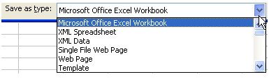
Save as type drop list

Saving Your Workspace

Sometimes you open one workbook. Other times, you might need to open several workbooks and switch between them. After you arrange the workbooks on your screen, consider using the Save Workspace command. The Save Workspace command saves the open workbooks plus their present location on your computer screen.

To use this command, click the File menu and choose Save Workspace. The Save Workspace dialog box opens, in the File Name box, type a name for the workspace file. Workspace files have the extension .XLW. Then click Save.

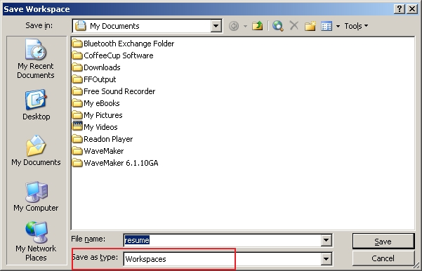
Save Workspace dialog box

You open a workspace file as you would any Excel file. Just click the Open button on the Standard toolbar, and double-click on the workspace file. Excel opens the file and arranges the workbooks the way you had saved them.

Auto Recovery

Excel also includes an Auto Recovery feature for accidental loss of work due to power failure or other mishap. When we start up again, the recovery file is automatically opened containing all changes we made up to the last time it was saved by auto recover.

Closing Workbook

On the File menu, click Close or use shortcut key combination – “Control” and “W” or click on Workbook close button in right end of menu bar.

Opening Workbook

Click File Menu than Open. If we want to open a workbook that was saved in a different folder, locate and open the folder. Double-click the workbook we want to open. If we can’t find the document in the folder list, we can search for it. The open dialog box is displayed in the figure below

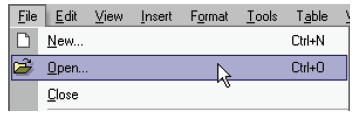
File Open Option

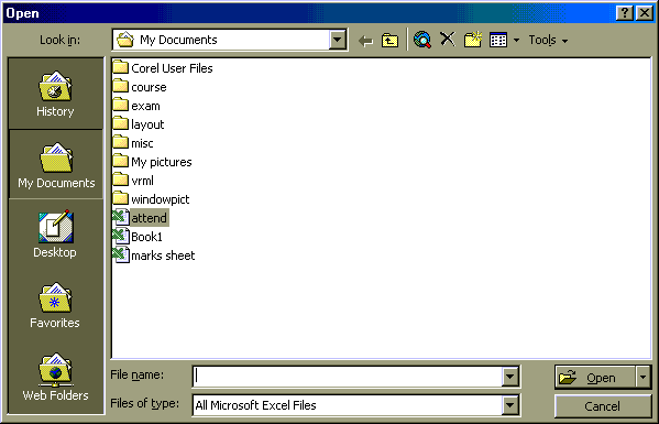
File Open dialog box

Exiting Excel

The exit command in the File Menu is used to quit the Excel program or click the X close button in the title bar. If we close without saving our document, excel displays a warning asking if we want to save our work. If we do not save our work and we exit, all our changes are lost. The keyboard shortcut is Alt + F4

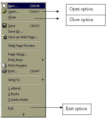
Selecting the Close option present in the File menu does quit a worksheet. If the exit option is selected than, MS-EXCEL closes all the open workbooks as well as closes the MS-EXCEL window. This illustrated by the figure –

Page Setup

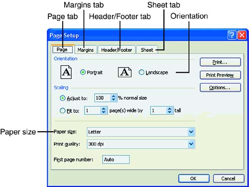
In Excel, you can print your worksheets just the way they look after you enter the data, or you can enhance the printout using several page layout options. When you select Excel’s Page Setup command, the Page Setup dialog box offers four tabs: Page, Margins, Header/Footer, and Sheet.

Orientation and Paper Size

The Page tab in the Page Setup dialog box is where you can change the page orientation and paper size. The two choices for page orientation are Portrait (vertical), which is the default, or Landscape (horizontal).

As for the paper size options, the default paper size is Letter (8.5×11), but you can choose Legal (8.5×14); Executive (7.25×10.5); A4, A5, and B5 (European sizes); envelopes; index cards; or a customized paper size.

Click the File menu and choose Page Setup. The Page Setup dialog box opens. You should see four tabs: Page, Margins, Header/Footer, and Sheet.

Page Setup dialog box

On the Page tab, change the orientation to landscape. In the Orientation area, click the Landscape option button.

Print the worksheet from the Page Setup dialog box. Click the Print button. The Print dialog box appears.

In the Print dialog box, click OK to print the worksheet. You should get a printout in landscape orientation on your 8.5×11-inch paper.

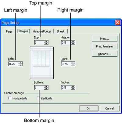
Changing the Page Margins

Margins are the empty spaces around the four edges of a page. Setting margins in Excel is very easy to do on the Margins tab in the Page Setup dialog box. You can change the margins before, during, or after you enter data in a worksheet.

Excel presets the top and bottom margins at 1″ and the left and right margins at 0.75.” You can adjust the margins for the top, bottom, left, and right sides of a page, as well as set the header and footer margins. The steps are

• Click the File menu and choose Page Setup. The Page Setup dialog box opens.
• Click the Margins tab. Excel shows you a sample page with the margin settings surrounding the page

• Change the left margin setting to 1″. In the Left box, click the up arrow once. The number 1 should appear in the box. This setting tells Excel to print the worksheet with a 1″ left margin.
• Change the right margin setting to 1″. In the Right box, click the up arrow once. The number 1 should appear in the box. Now Excel knows to print the worksheet with a 1″ right margin.
• Print the worksheet from the Page Setup dialog box. Click the Print button. The Print dialog box appears.
• In the Print dialog box, click OK to print the worksheet. Your worksheet should print with 1″ left and right margins.

Printing Gridlines

By default, Excel worksheets print without gridlines, which separate the cells as it looks cleaner without the grids. However, to change overall appearance of worksheet by printing the gridlines follow the steps

• Click the File menu and choose Page Setup.
• In Sheet tab click Gridlines check box to put a check mark in the box.
• Print the worksheet from the Page Setup dialog box. Click the Print button.
• Click OK in the Print dialog box to print the worksheet. Worksheet will print with gridlines.

Headers and Footers

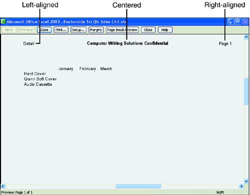
Headers and footers are lines of text that you can print at the top and bottom of every page in a print job—headers at the top, footers at the bottom. You can include any text, the current date and time, or the filename, and you can even format the information in a header and footer. Excel also gives you a variety of preset headers and footers to choose from in case you don’t want to create your own. A header is a line or several lines of text that appears at the top of each page just below the top margin. Footer is a line or several lines of text that appears at the bottom of each page just below the bottom margin. We can select from predefined header and footer text or enter our own custom text. The information contained in the predefined header and footer text is taken from the document properties associated with the worksheet and from the program and system settings. Header and footer text can be formatted like any other text. In addition, we can control the placement of the header and footer text by specifying where it should appear: left aligned, centered, or right-aligned in the header or footer space. Information that is commonly placed in a header or footer includes the date and page number.

Preset Headers and Footers

Because a workbook can contain multiple worksheets, you might need to reference a cell in another worksheet, or even another workbook file. No problem! As long as you follow the proper syntax, you can type a formula that contains a reference to any file.

The default header is (none).

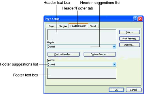
Click the Header down arrow, and a list of suggested header information appears. Scroll through the list to Detail, and then click it. The sample header appears centered at the top of the Header box.

By default, the footer (none) appears in the Footer text box. Click the Footer down arrow, and a list of suggested footer information appears. Scroll through and then click it. The sample footer appears centered at the bottom of the Footer box. Click OK.

To see the header and footer, click the Print Preview button on the Header/Footer tab of the Page Setup dialog box. It displays header and footer.

Custom Headers and Footers

To customize a header or footer, in File menu, click Page Setup and select Header/Footer tab if necessary.

Click the Header down arrow, scroll to the top of the list to None and then click it. The Header text box should now be empty.

Click the Custom Header button. The Header dialog box opens. It contains buttons for formatting the header text. Three boxes are visible: Left Section, Center Section, and Right Section to place custom text in either end of the header.

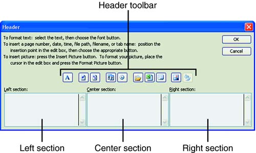
Type your custom text and click OK. Similarly give custom text for footer.

To see the header and footer, click the Print Preview button on the Header/Footer tab of the Page Setup dialog box.

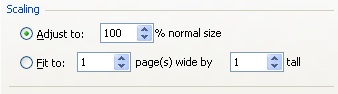
Scaling

We can scale the content to be printed either scale down or up depending upon the need. In the page setup option of File menu, click page tab and then in scaling section we can customize the zoom level. As in the figure

Scale level

Printing

Excel gives you several ways to print a worksheet

• Select File, Print.
• Press Ctrl+P.
• Click the Print button on the Standard toolbar.

When you select File, Print or press Ctrl+P, Excel displays the Print dialog box. This dialog box enables you to print some or all the pages within a worksheet, selected data, the active worksheet, or the entire workbook. You can also specify the number of copies of the printout, and you can collate pages when you print multiple copies of a multi page worksheet. You can even print a worksheet to another file.

Before you use your printer with Excel, it’s advisable to check the Printer options which let you select the paper size and paper type. You can choose the paper feed type: cut-sheet (single sheets of paper) or banner (continuous form paper). You can also select from three types of print quality

Best— Highest quality, slower printing than Normal mode; uses more ink.

Normal— Letter quality; normal printing speed.

EconoFast— Draft quality, lighter output, faster printing than Normal mode. Uses less ink than other modes and reduces the frequency of replacing your print cartridges; available only when you select Plain Paper as the paper type.

Printing Single Worksheet

If you want to print one worksheet just the way it is without changing any print options, simply click the Print button on the Standard toolbar. But suppose you want to print more than one worksheet. No problem—you just need to tell Excel which worksheets you want to print. You can print contiguous or noncontiguous worksheets.

• Contiguous worksheets—Worksheets that are next to each other in the workbook, without any worksheet that you don’t want in between them.
• Noncontiguous worksheets—Worksheets that are separated by several worksheets that you do not want.

Printing a Range

You can choose which pages you want to print in the Print Range area in the Print dialog box. You have two choices: All or Pages. Printing all the pages in your active sheet is the default print range setting. However, you can print specific pages by choosing the Page(s) option and entering the page numbers in the From and To boxes.

Printing a Selection

To print a portion of the worksheet select the cells, rows, and/or columns you want to print. Then click File, Print. In the Print dialog box, in the Print this option prints only the portion of the worksheet you selected.

Printing the Entire Workbook

You can print the entire workbook with all its worksheets in one step. In File menu, Click Print option. In the Print dialog box, choose Entire Workbook. This option prints the whole workbook.

Printing Selection

We can also print only a portion of the worksheet, and not the whole worksheet or workbook. Excel’s Print Area feature lets you single out an area on the worksheet that you want to print. The Print Titles feature lets you repeat the title, subtitle, column headings, and row headings on every page.

Excel’s Fit To option lets you shrink the pages to fit any number of pages you want by shrinking a worksheet down so small that you can’t read the text. If you shrink it to some suitable multiple-page setting, such as 1 page wide by 3 pages high, you could read the text comfortably.

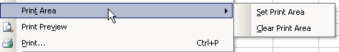
Set Print Area

To select the print area, highlight the cells that contain the data. Don’t highlight the column and row headings. Next in File menu, in Print Area drop down menu click on Set Print Area. Excel inserts automatic page breaks to the left and right and the top and bottom of the range you selected. You should see a dashed line border around the print area. To remove the print area, click File, Print Area, and Clear Print Area. The automatic page breaks should disappear in the worksheet.

Print area selection

Printing Column and Row Headings

You can select titles that are located on the top edge (column headings) and left side (row headings) of your worksheet and print them on every page of the printout. The steps are –

• Click File, Page Setup and click the Sheet tab. You see the Sheet options.
• Click in the Rows To Repeat At Top text box.
• Click in worksheet and select and drag to include the title, subtitle, and column headings to repeat.
• Click in the Columns to Repeat at Left text box.
• Click on any cell in column A to include the row headings.
• Click OK to confirm your choices. All data above and to the left of the dashed-line border (print area) repeat on every page.

To remove the repeated row and columns headings, delete the values in the Rows to Repeat at Top and Columns to Repeat at Left boxes on the Sheet tab in the Page Setup dialog box.

Fitting Your Worksheet to a Number of Pages

If you have a large worksheet divided into several pages, you can shrink the pages to fit on one page by using the Fit To option. For instance, if the worksheet is two pages wide by three pages tall, you can reduce the worksheet to fit on one page by selecting the Fit To option. Because the default setting for this option is one page wide by one page tall, Excel prints your worksheet on one page. Steps for the option are

• Click the File menu and choose Page Setup.
• Click the Page tab. In the Scaling section, choose the Fit To option.

Page Break

If your worksheet is too large to fit on one page, Excel splits the work over two or more pages. Excel makes the split based on your current page dimensions, margins, and cell widths and heights. Excel always splits the worksheet at the beginning of a column (vertically) and/or row (horizontally), so the information in a cell is never split between two pages.

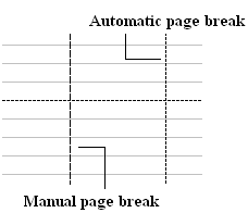
An automatic page break appears as a dashed line with short dashes in your worksheet. These dashed lines run down the right edge of a column.

If the automatic page breaks are not right for your worksheet, one of the many ways to make adjustments is to override Excel’s defaults. The worksheet still prints on two or more pages, but you can control where each new page begins.

Manual Page Break

To set a page break, click in any cell, row, or column where you want the break to appear. Click the Insert menu and choose Page Break. Excel inserts a manual page break, which is indicated by a dashed line. Onscreen, manual page breaks have longer, thicker dashed lines than automatic page breaks

If you’re using the Fit To page setup option, the manual page break does not appear.

To remove a manual page break, just select the cell, row, or column that was used to create the break and choose Insert, Remove Page Break.

Moving around a worksheet

To move between cells on a worksheet, click any cell or use the arrow keys. When we move to a cell, it becomes the active cell. To see a different area of the sheet, use the scroll bars.

To scroll	Do this
One row up or down	Click the arrows in the vertical scroll bar.
One column left or right	Click the arrows in the horizontal scroll bar.
One window up or down	Click above or below the scroll box in the vertical scroll bar.
One window left or right	Click to left or right of scroll box in the horizontal scroll bar.
A large distance	Drag the scroll box to the approximate relative position. In a very large worksheet, hold down SHIFT while dragging