Factor analysis is a statistical method used to describe variability among observed, correlated variables in terms of a potentially lower number of unobserved variables called factors. For example, it is possible that variations in four observed variables mainly reflect the variations in two unobserved variables. Factor analysis searches for such joint variations in response to unobserved latent variables. The observed variables are modeled as linear combinations of the potential factors, plus “error” terms. The information gained about the interdependencies between observed variables can be used later to reduce the set of variables in a dataset. Computationally this technique is equivalent to low-rank approximation of the matrix of observed variables. Factor analysis originated in psychometrics and is used in behavioral sciences, social sciences, marketing, product management, operations research, and other applied sciences that deal with large quantities of data.
Factor analysis is related to principal component analysis (PCA), but the two are not identical. Latent variable models, including factor analysis, use regression modeling techniques to test hypotheses producing error terms, while PCA is a descriptive statistical technique. There has been significant controversy in the field over the equivalence or otherwise of the two techniques.
The key concept of factor analysis is that multiple observed variables have similar patterns of responses because they are all associated with a latent (i.e. not directly measured) variable. For example, people may respond similarly to questions about income, education, and occupation, which are all associated with the latent variable socioeconomic status.
In every factor analysis, there are the same number of factors as there are variables. Each factor captures a certain amount of the overall variance in the observed variables, and the factors are always listed in order of how much variation they explain.
The eigenvalue is a measure of how much of the variance of the observed variables a factor explains. Any factor with an eigenvalue ≥1 explains more variance than a single observed variable.
So if the factor for socioeconomic status had an eigenvalue of 2.3 it would explain as much variance as 2.3 of the three variables. This factor, which captures most of the variance in those three variables, could then be used in other analyses.
The factors that explain the least amount of variance are generally discarded. Deciding how many factors are useful to retain will be the subject of another post.
Factor Loadings
The relationship of each variable to the underlying factor is expressed by the so-called factor loading. Here is an example of the output of a simple factor analysis looking at indicators of wealth, with just six variables and two resulting factors.
| Variables | Factor 1 | Factor 2 |
| Income | 0.65 | 0.11 |
| Education | 0.59 | 0.25 |
| Occupation | 0.48 | 0.19 |
| House value | 0.38 | 0.60 |
| Number of public parks in neighborhood | 0.13 | 0.57 |
| Number of violent crimes per year in neighborhood | 0.23 | 0.55 |
The variable with the strongest association to the underlying latent variable. Factor 1, is income, with a factor loading of 0.65. Since factor loadings can be interpreted like standardized regression coefficients, one could also say that the variable income has a correlation of 0.65 with Factor 1. This would be considered a strong association for a factor analysis in most research fields.
Two other variables, education and occupation, are also associated with Factor 1. Based on the variables loading highly onto Factor 1, we could call it “Individual socioeconomic status.”
House value, number of public parks, and number of violent crimes per year, however, have high factor loadings on the other factor, Factor 2. They seem to indicate the overall wealth within the neighborhood, so we may want to call Factor 2 “Neighborhood socioeconomic status.” The variable house value also is marginally important in Factor 1 (loading = 0.38). This makes sense, since the value of a person’s house should be associated with his or her income.
Definition
Suppose we have a set of observable random variables, ![]() with means
with means ![]() Suppose for some unknown constants
Suppose for some unknown constants ![]() and
and ![]() unobserved random variables
unobserved random variables ![]() where
where ![]() and
and ![]() , where
, where ![]() , we have
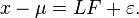
, we have

Here, the are independently distributed error terms with zero mean and finite variance, which may not be the same for all í Let ![]() so that we have
so that we have

In matrix terms, we have
If we have η observations, then we will have the dimensions ![]() and
and ![]() . Each column of
. Each column of ![]() and
and ![]() denote values for one particular observation, and matrix
denote values for one particular observation, and matrix ![]() does not vary across observations.
does not vary across observations.
Also we will impose the following assumptions on ![]()
 and are independent.
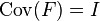 (to make sure that the factors are uncorrelated).

Any solution of the above set of equations following the constraints for ![]() is defined as the factors, and
is defined as the factors, and ![]() as the loading matrix. Suppose
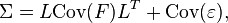
as the loading matrix. Suppose ![]() . Then note that from the conditions just imposed on
. Then note that from the conditions just imposed on![]() , we have
, we have
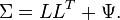
or
or
For any orthogonal matrix ![]() if we set
if we set ![]() and
and ![]() ,the criteria for being factors and factor loadings still hold. Hence a set of factors and factor loadings is identical only up to orthogonal transformation.
,the criteria for being factors and factor loadings still hold. Hence a set of factors and factor loadings is identical only up to orthogonal transformation.
Example
The following example is for expository purposes, and should not be taken as being realistic. Suppose a psychologist proposes a theory that there are two kinds of intelligence, “verbal intelligence” and “mathematical intelligence”, neither of which is directly observed. Evidence for the theory is sought in the examination scores from each of 10 different academic fields of 1000 students. If each student is chosen randomly from a large population, then each student’s 10 scores are random variables. The psychologist’s theory may say that for each of the 10 academic fields, the score averaged over the group of all students who share some common pair of values for verbal and mathematical “intelligences” is some constant times their level of verbal intelligence plus another constant times their level of mathematical intelligence, i.e., it is a combination of those two “factors”. The numbers for a particular subject, by which the two kinds of intelligence are multiplied to obtain the expected score, are posited by the theory to be the same for all intelligence level pairs, and are called “factor loadings” for this subject. For example, the theory may hold that the average student’s aptitude in the field of taxonomy is
{10 × the student’s verbal intelligence} + {6 × the student’s mathematical intelligence}.
The numbers 10 and 6 are the factor loadings associated with taxonomy. Other academic subjects may have different factor loadings. Two students having identical degrees of verbal intelligence and identical degrees of mathematical intelligence may have different aptitudes in taxonomy because individual aptitudes differ from average aptitudes. That difference is called the “error” — a statistical term that means the amount by which an individual differs from what is average for his or her levels of intelligence (see errors and residuals in statistics).
The observable data that go into factor analysis would be 10 scores of each of the 1000 students, a total of 10,000 numbers. The factor loadings and levels of the two kinds of intelligence of each student must be inferred from the data.
