In Discrete Probability Distributions, with each experiment that is considered there will be associated a random variable, which represents the outcome of any particular experiment. The set of possible outcomes is called the sample space. Firstly, one has to consider the case where the experiment has only finitely many possible outcomes, i.e., the sample space is finite. Then, it is generalized to the case that the sample space is either finite or countably infinite. This leads to the following definition.
Random Variables and Sample Spaces
Suppose there is an experiment whose outcome depends on chance. The outcome of the experiment is represented by a capital Roman letter, such as X, called a random variable. The sample space of the experiment is the set of all possible outcomes. If the sample space is either finite or countably infinite, the random variable is said to be discrete.
Generally a sample space is denoted by the capital Greek letter Ω. As stated above, in the correspondence between an experiment and the mathematical theory by which it is studied, the sample space Ω corresponds to the set of possible outcomes of the experiment.
Two additional definitions- These are subsidiary to the definition of sample space and serve to make precise some of the common terminology used in conjunction with sample spaces.
- First of all, the elements of a sample space is defined to be outcomes.
- Second, each subset of a sample space is defined to be an event . Normally, outcomes are denoted by lower case letters and events by capital letters.
Example – A die is rolled once. We let X denote the outcome of this experiment. Then the sample space for this experiment is the 6-element set
Ω = {1, 2, 3, 4, 5, 6} ,
where each outcome i, for i = 1, …, 6, corresponds to the number of dots on the face which turns up. The event
E = {2, 4, 6}
corresponds to the statement that the result of the roll is an even number. The event E can also be described by saying that X is even. Unless there is reason to believe the die is loaded, the natural assumption is that every outcome is equally likely. Adopting this convention means that we assign a probability of 1/6 to each of the six outcomes, i.e., m(i) = 1/6, for 1 ≤ i ≤ 6.
Distribution Functions
Assignment of probabilities- The definitions are motivated by the example above, in which each outcome of the sample space was assigned a nonnegative number such that the sum of the numbers assigned is equal to 1.
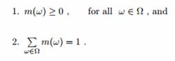
Let X be a random variable which denotes the value of the outcome of a certain experiment, and assume that this experiment has only finitely many possible outcomes. Let Ω be the sample space of the experiment (i.e., the set of all possible values of X, or equivalently, the set of all possible outcomes of the experiment.) A distribution function for X is a real-valued function m whose domain is Ω and which satisfies
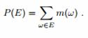
For any subset E of Ω, we define the probability of E to be the number P (E) given by
Binomial Distribution
It is used to model discrete data having only two possible outcomes like pass or fail, yes or no and which are exactly two mutually exclusive outcomes. It may be used to find the proportion of defective units produced by a process and used when population is large – when N> 50 with small size of sample compared to the population. The ideal situation is when sample size (n) is less than 10% of the population (N) or n< 0.1N. The binomial distribution is useful to find the number of defective products if the product either passes or fails a given test. The mean, variance, and standard deviation for a binomial distribution are µ = np, σ2= npq and σ =√npq. The essential conditions for a random variable are fixed number of observations (n) which are independent of each other, every trial results in either of the two possible outcomes and if the probability of a success is p and the probability of a failure is 1 -p.
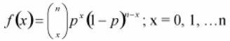
The binomial probability distribution equation will show the probability p (the probability of defective) of getting x defectives (number of defectives or occurrences) in a sample of n units (or sample size) as
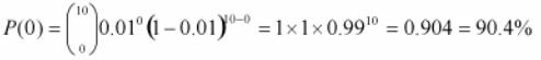
As an example if a product with a 1% defect rate, is tested with ten sample units from the process, Thus, n= 10, x= 0 and p= .01 then, the probability that there will be 0 defective products is
Poisson Distribution
It estimates the number of instances a condition of interest occurs in a process or population. It focuses on the probability for a number of events occurring over some interval or continuum where µ, the average of such an event occurring, is known like project team may want to know the probability of finding a defective part on a manufactured circuit board. Most frequently, this distribution is used when the condition may occur multiple times in one sample unit and user is interested in knowing the number of individual characteristics found like critical attribute of a manufactured part is measured in a random sampling of the production process with non-conforming conditions being recorded for each sample. The collective number of failures from the sampling may be modeled using the Poisson distribution. It can also be used to project the number of accidents for the following year and their probable locations. The essential condition for a random variable to follow Poisson distribution is that counts are independent of each other and the probability that a count occurs in an interval is the same for all intervals. The mean and the variance of the Poisson distribution are the same, and the standard deviation is the square root of the mean hence, µ = σ2 and σ =√µ =√σ2.
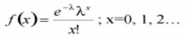
The Poisson distribution can be an approximation to the binomial when p is equal to or less than 0.1, and the sample size n is fairly large (generally, n >= 16) by using np as the mean of the Poisson distribution. Considering f(x) as the probability of x occurrences in the sample/interval, λ as the mean number of counts in an interval (where λ > 0), x as the number of defects/counts in the sample/interval and e as a constant approximately equal to 2.71828 then the equation for the Poisson distribution is as
Geometric distribution
It addresses the number of trials necessary before the first success. If the trials are repeated k times until the first success, we would have k−1 failures. If p is the probability for a success and q the probability for a failure, the probability of the first success to occur at the kth trial is P(k, p) = p(q)k−1 with the mean and standard deviation are µ =1/p and σ = √q/p.
Hypergeometric Distribution
The hypergeometric distribution applies when the sample (n) is a relatively large proportion of the population (n >0.1N). The hypergeometric distribution is used when items are drawn from a population without replacement. That is, the items are not returned to the population before the next item is drawn out. The items must fall into one of two categories, such as good/bad or conforming/nonconforming.
The hypergeometric distribution is similar in nature to the binomial distribution, except the sample size is large compared to the population. The hypergeometric distribution determines the probability of exactly x number of defects when n items are samples from a population of N items containing D defects. The equation is
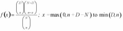
With, x is the number of nonconforming units in the sample (r is sometimes used here if dealing with occurrences), D is the number of nonconforming units in the population, N is the finite population size and n is the sample size.
