Classical EOQ Model
In this section we discuss some elementary inventory models with deterministic demand and lead time situations. The purpose is to provide an illustration of the mathematical analysis of inventory systems. The most classical of the inventory models was first proposed by Harris in 1915 and further developed by Wilson in 1928. It is very popularly known as EOQ (Economic Order Quantity) model or ‘Wilson’s Lot Size formula’.
When dealing with stocked items, the two important decisions to be made are-how much to order and when to order. EOQ attempts to provide answer to former while the Reorder point (RoP) provides the answer to the latter.
The following assumptions are made in the standard Wilson lot size formula to obtain EOQ:
- Demand is continuous at a constant rate
- The process continues infinitely.
- No constraints are imposed on quantities ordered, storage capacity, budget etc.
- Replenishment is instantaneous (the entire order quantity is received all at one time as soon as the order is released).
- All costs are time-invariant.
- No shortages are allowed
- Quantity discounts are not available.
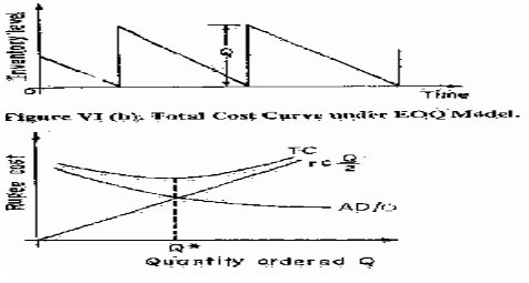
The inventory status under EOQ-RoP policy is continuously reviewed. Figure VI (a) shows the behavior of such a simple system whereas Figure VI (b) shows the total system cost behavior highlighting the conflicting trend of ordering and inventory carrying costs. EOQ aims at minimizing total system cost. ~
Let us use the following notation in developing the classical EOQ model: Inventory Management D = Demand rate; unit per year.
A = Ordering cost; Rs./order.
C = Unit cost, Rs. per unit of item.
r = Inventory carrying charge per year.
H = Annual cost of carrying inventory/unit item = r.c.
TC = Total annual cost of operating the system Rs./year (objective function).
Q = Order quantity, Number of units per lot (decision variable).
Since demand is at uniform rate average inventory is Q/2 throughout the year and the total number of orders are (D/Q) per year. Thus total annual cost of operating the systems consisting of carrying cost and ordering cost can be written as:
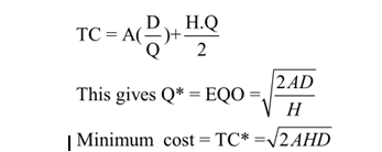
Due to convex nature of total cost curve, it is obvious that Q * (EOQ) gives the global minimum total cost. It can also be seen that EOQ is obtained at the point of intersection of ordering cost and carrying cost in Figure VI (b).
Some interesting insight may be obtained using this classical system:
- If ordering cost is of high tendency, the optimal policy is to have high EOQ thus raising average inventory level.
- If r or care high leading to high value of H, the tendency will be to go for smaller lot sizes.
r may vary from 0.15-0.30 and will depend on the nature of item, A the ordering cost should be marginal ordering cost while H should be based on total purchased cost of the items.
Finite Replenishment Rates
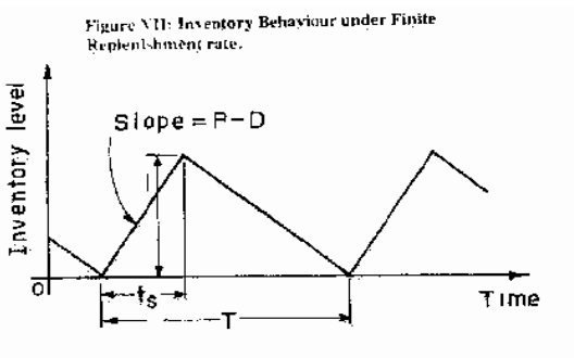
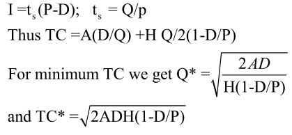
We will now relax the assumption (d) of the classical EOQ model and permit finite replenishment rate (staggered deliveries). When the rate of procurement is P in units/year and the demand rate is D, in units/year, the buildup of inventory is at a rate (P-D) due to simultaneous consumption. It is obvious that P> .D for inventory to build up. Figure VII shows the inventory behavior with finite supply rate. The stock builds up to a maximum level I during supply period ts, after which stock depletion takes place at rate D. It can be seen that
Some interesting observations can be made about the behaviour of such systems. These are:
- Q* under finite replenishment rates are higher than Q* under classical EOQ model for the same values of other parameters.
- Total system cost under optimal Q* is lower than corresponding total system cost and EOQ model.
- Thus staggering the supplies always reduces inventory level and total operating system cost provided other cost parameters remain the same.
- As P–>∞,Q* and TC* obtained are same as in standard Wilson’s formula of instantaneous replenishment.
- At P = D, Q*.–>∞ TC->0. Thus if we can have a fully devoted reliable supplier, then placing a single supply order of large size but matching supply rate with the demand rate is the optimal decision. Under such a system, no .stocks is built, no replenishments are made, and no shortages are incurred. This would seem to be an ideal system towards zero-inventory provided we know our requirements for sure and we have a dependable source to supply us at the rate to match the requirement. This brings out the role of dependable source of supply as an important asset to materials management function.
Planned Backlogging
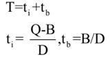
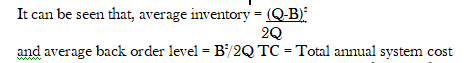
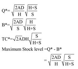
Let us now consider the effect of relaxing assumption (f) of classical Wilson’s model by permitting backlogging (shortages or back ordering) at a unit shortage cost of S in Rs./unit short/year. In such a case negative inventory shows the backlogging position. The order quantity Q is partly used to clear the backlogging level B and (Q-B) is the maximum stock level. Figure VIII shows the inventory behavior under planned backlogging Inventory is maintained for duration ti and demands remain backlogged for duration tb. Total cycle time of each replenishment cycle is
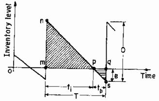
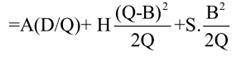
optimal values of Q and B can be obtained for minimum value of TC as follows:
Some useful observations could be made about the behavior of inventory system with planned backlogging as follows:
- Total system cost is lower with planned backlogging than the corresponding total system cost under classical Wilson’s lot size formula. Thus for a deterministic system with finite backlogging cost, it is economical to plan for backlogging. It can be seen that at S->∞, the model reverts to classical EOQ model.
- EOQ under backlogging is higher and maximum stock level is lower than the corresponding values under classical Wilson’s lot size model.
- If S = 0 then B* = Q* = co. This means that with no charge for back orders one would keep piling up unfilled demand until the backlog gets infinitely large. Then one single order would be released to satisfy all accumulated demand. However, considering intangible cost of backordering such as loss of goodwill etc. it is debatable whether there are situations when the unit cost of shortages (S) is really zero.
Model with Quantity Discounts
Frequently, the vendors offer quantity discounts on bulk purchases to encourage users to place orders in large quantities. Quantity discounts may be all unit discounts or incremental quantity discounts. In all unit discounts entire order quantity is purchased at lower unit price if order size is higher than or equal to the stipulated conditions. In incremental case only quantity exceeding the threshold point is charged at lower unit cost. The immediate reaction may be to avail the discount and place bulk orders but if we see the total system cost, our decision may be otherwise. There may be a single or multiple quantity discounts. Figure IX shows total system costs under four discounts.
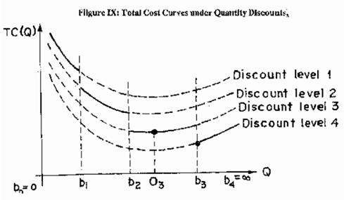
The broken lines show the total cost curves without price break whereas solid lines show the actual total cost if price break takes place. The larger the number of price breaks, the more difficult it becomes to analyze the situation as more alternatives are to be evaluated. The important point to be made in such situations is that individual tuition is to be analyzed to judge which of the options is suitable to avail discount and place bulk order to make it realizable, reject the offer and place small order at higher unit price or place order at the minimum possible quantity at which discount becomes valid. Any alternative is optimal if that minimizes the total system cost. For example, it can be easily seen from Figure IX that for this case the minimum total system cost occurs at Q* = b3 is the minimum quantity at which discount level 4 is applicable.
Sensitivity Analysis
It may not be operationally very convenient to stick to EOQ if it is an odd figure. Then one may like to know the repercussions on total system cost if one deviated either way from Q*. This is done through sensitivity analysis. If Qa is actual order quantity, Qa = b.Q* where b is sensitivity parameter. If b = 0.8 then actual Qa is 20% less than Q* and if b = 1.2 then Qa is 20% less of higher than Q*. Obviously the TC will increase over TC* in either case. If we substitute Qa as bQ* in total cost expressions in the classical EOQ model, we can easily get the following relationship.
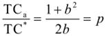
Where TCa is actual cost with order size being Qa It can be seen that at b = 1, p = 1. If b is allowed to vary within 0.9 to 1.10 then p will be within 1.005 indicating that ±10% deviation in EOQ leads to less than half a per cent increase in TC Thus TC is not very sensitive to EOQ and for operational convenience we should be able to vary EOQ within ± 10% of Q* without adversely affecting total system cost.
