Decision Trees are most commonly used in capacity planning. They are excellent tools for helping choose between several courses of action. They provide an effective structure within which you can lay out options and investigate the possible outcomes of choosing those options. They also provide a balanced picture of the risks and rewards associated with each possible courses of action.
The capacity planning exercise requires methods by which alternative options are evaluated. Two metrics are useful to perform the evaluation. In the cost based methods, each alternative can be evaluated from the perspective of cost and benefits accruing out of the alternative. A firm, for example, may be considering three options: not to do anything about capacity, add a new machine or go for sub-contracting. Another firm may have three options of varying technological and operational capabilities for capacity addition, resulting in different capital costs, operating costs and useful life of the resource. In each of the above examples, one can evaluate the alternatives from the perspective of costs and benefits.
The other method is to use operational performance based methods for comparing alternatives. If the choice is to go for multiple resources, one can analyze the impact of the alternatives in terms of utilization of capacity and the waiting time of the jobs. If more machines are added, the waiting time as well as the utilization of the resource will come down. It is possible to analyze and select the best alternative on the basis of these measures.
Decision trees are useful to evaluate alternative capacity choices on the basis of cost of the capacity and the benefits. Further, the inherent uncertainty in the demand tree is a schematic model in which different sequences and steps involved in a problem and the consequences of the decisions are systematically portrayed. Decision trees comprise nodes and branches. Each node represents the decision point and branches represent the potential outcomes of the decision. The consequence of each outcome is measured as the cost of the impact, and the uncertainty associated with each outcome could be associated with the requisite branch. Using this basic information, the tree is constructed. After the tree is constructed, each branch in the tree is evaluated with respect to the costs, benefits and uncertainty. The tree is evaluated from right to left (from end to beginning). As we move from right to left, unattractive portions of the tree are eliminated to arrive at the final decision. The used of a decision tree for evaluating capacity alternatives is explained with the help of an example below.
Waiting Line Models: Consider the capacity planning in the case of the computerized passenger reservation facility of Indian Railways. In simple terms, the question boils down to deciding the number of booking counters to be made available to the public. It is obvious that if there are fewer booking counters to be made available to the public. It is obvious that if there are fewer booking counters, the queue is likely to build and customers may end up spending more time in the system before they get their tickets booked. We have similar experiences in a banking system or BSNL’s bill payment counters. Capacity decisions in service systems are often made on the basis of the impact on the customers. In service systems, waiting time is an important operational measure that determines service quality. Similar examples exist in manufacturing systems as well. A resource that is few in number and highly utilized is likely to be a bottleneck and increase the waiting time of the jobs ahead of it. Due to this, manufacturing lead time will increase and work in progress will pile up in the factory. This will have a cascading effect in terms of missing delivery commitments and shipping delays.
Waiting line models make use of queuing theory fundamentals such as queue length, waiting time and utilization of resources, to analyze the impact of alternative capacity choices on important operational measures in operating systems. Therefore, capacity planning problem could be analyzed using queuing system and the alternative scenarios that can be analyzed that can be analyzed using the waiting line models developed.
Basic Structure of a Queuing System: Figure 4.3 depicts the basic structure of a queuing system. The demand for the products/ services offered by the operating system originates from a calling population or source. In the case of a restaurant, the calling population (source) of demand could be the citizens in the vicinity of the restaurant. The demand manifests in the form of arrivals at the system. In the case of service systems it could be actual customers arriving to get the service. In the case of a manufacturing system it could be work orders at a shop or customer orders at a division. The third element is the waiting line, which characterizes the provisions made for the arrivals to wait for their turn. There are servers in the system for service delivery and finally the served customers exit the system. We shall understand each element in details and enumerate alternative representations that exist in real life in each of these. Figure 4.3 provides the elements of waiting line models in a nutshell and enumerates the alternatives pertaining to each element.
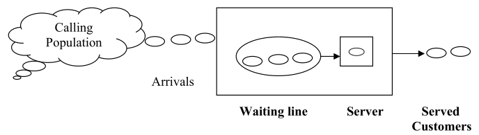
Fig. 4.3Basic Structure of a Queuing System
Calling Population: It is the calling population in an operating system that places a demand and uses the capacity deployed. In several cases the calling populating is infinite for all practical purposes. For instance, the calling population for a petrol bunk in the city of Delhi could be the entire set of vehicles running on the roads of Delhi. Similarly for a bank in a metropolitan city such as Chennai the calling population could be the individual and institutional members in the society in the city. These typically amount to an infinite number as far as the operating system is concerned. However, in some cases, the calling population could be finite. Consider the maintenance department in a large manufacturing plant. If there are 300 machine tools in the plant, they form the calling population for the maintenance department in the manufacturing plant. Every machine breakdown corresponds to an arrival at the maintenance shop. In this situation, the calling population is finite. The important difference between an infinite source and a finite one is the manner in which arrival rates are estimated. Clearly, every arrival from a calling population decreases the probability of arrival of the remaining machines at the maintenance shop.
