
The CAPM was developed to explain the riskiness of securities priced in the market and this was attributed to experts like Sharpe and Lintner. Markowitz theory being more theoretical, CAPM aims at a more practical approach to stock valuation.
CAPM-Assumptions
The CAPM is based on certain assumptions. These assumptions (few in common with Market Portfolio Theory) are set out below.
The investor aims at maximizing the utility of his/her wealth, rather than the wealth or rerun. The difference between them is that individual preferences are taken into account in the utility concept. While some have the capacity for larger risk and will have increasing marginal, utility for wealth for others with less capacity for risk, the incremental wealth will be less attractive if it is attached with more risk. Thus, the preference of investors for risk return is taken into account in this model.
Investors have similar expectations of Risk and Return. Without these consensus standards, the estimates of mean and variance may lead to different forecasts with the result that the client portfolio of each will be different from that of the others. There will be innumerable efficient frontiers, each dependent on the set of preferences of individuals for risk and return. If investors do not have similar expectations there will be no homogeneity in their conception and no single efficient frontier line will apply to all.
This in turn will imply that the price of an asset, which is the best estimate of the present value of future returns, will be different for different investors.
- Investors make investment decision on a rational basis, depending on their assessment of risk and return. Risk is measured by two factors, mean and variance. In the CAPM it is assumed that rational investors diversify away their diversifiable risk, namely, unsystematic risk and only systematic risk remains which varies with the Beta of the security.
- While some use only the beta as a measure of risk, others use both beta and variance of returns (total Risk) as the sources of reward or expected return. As these perceptions of risk and reward vary from individual to individual, there are a series of efficient frontier lines in CAPM while in the case of MPT, there will be a single efficient frontier line as the conception of risk and return expectation is assumed to be homogeneous in the latter.
- Investors will have free access to all available information at no cost and no loss of time.
- The transactions cost is low enough to ignore and assets can be bought and sold in any unit desired. The investor is limited only by his wealth and the price of the asset.
- Taxes do not affect the buying of assets.
- Investors should have identical time horizons. Investors make their investment decisions based on a single period horizon.
The assumptions above enable managers to be much more precise about how trade-offs between risk and returns are understood in the financial market.
In the CAPM, the expected rate of return is taken as the ‘required rate of return’ because the market is believed to be in equilibrium. The expected return is the return from an asset that investors anticipate over a future period. The required rate of return is the minimum expected rate of return needed to induce an investor to purchase it.
Elements of CAPM
- Capital Market Line: Risk returns relationship for efficient portfolios.
- Security Market Line: Graphic representation of CAPM and market price of risk in capital markets.
- Risk Return Relationship
- Risk Free Rate
- Risk Premium on market portfolios
- Beta: Measure the risk of an individual asset value to market portfolio. Assets
- Defensive Assets
- Aggressive Assets
After the brief review of the above assumptions, the requirements for CAPM can be summarized as follows.
Risk is measured by variance of expected returns. There are two components of Risk – systematic (non-diversifiable) and unsystematic (diversifiable). For diversifiable risk, the investor makes a proper diversification to reduce the risk and for the non-diversifiable portion, he/she uses the relevant Beta measure to adjust to his requirement or preferences.
Due to the possibility of risk free asset and lending and borrowing at the free rate, the investor has two components of the portfolio – risk free assets and the risky market assets. The total return is a summation from the above two components. CAPM establishes a linear relationship between the required rate of return of a security and its systematic risk (beta). It is represented as.
kj = Rf + Bj (km – Rf)
Where
kj = expected or required rate of return on security j
Rf = risk-free rate of return
Bj = Beta coefficient of security j
km= return on market portfolio
Under CAPM, the equilibrium situation arises when all frictions, like taxes, divisibility transaction costs and different risk-free borrowing and lending rates are assumed away. Equilibrium will be brought about by changes in prices due to changes in demand and supply.
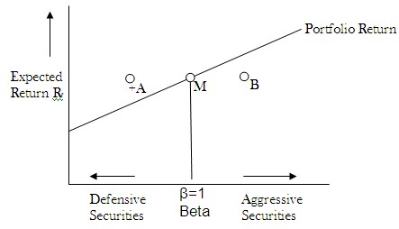
Security Market Line (SML)
Security market line, also known as characteristic line is the graphical representation of Capital Asset Pricing Model or CAPM. Security market line is a straight slopping line which gives the relationship between expected rate of return and market risk (or systematic risk) of the overall market.
The X-axis of the security market line represents the market risk or beta and the Y-axis of SML represents expected market return in percentage at a point of time. Usually the rate of risk free investments is represented as a line parallel to X-axis and it is from here that the SML starts.
Example
The risk-free ratio is 4%, the beta value of market is 3% and expected return from market is 10%.
The expected return.
= 4 + 3(10 – 4) = 22%
SML will start from 4% at Y-axis and will pass through 22% when beta is 3.
Investors can plot individual stock’s beta and expected return against SML. If the expected return from the stock is above SML the stock is considered undervalued and is predicted to offer good return for the risk taken. If the expected return falls below SML, the stock is considered overvalued and is predicted to offer lesser return for the risk taken.
Security Market Line

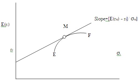
The Capital Market Line (CML)
The capital market equation depicts the expected return of a two asset portfolio, consisting of one risk free asset and one risky asset. With the ability to borrow and lend at the risk-free rate ri, in conjunction with an investment in market portfolio M, the old curved efficient frontier is transformed into a new efficient frontier, which is a line passing from ri, through market portfolio M. This new linear efficient frontier is called the Capital Market Line. The CML also expresses the equilibrium pricing relationship between E(r) and σ for all efficient portfolios lying along the line.
The CML relationship for any portfolio i can be determined using:
E (ri) = rf + {[E (rM) – rf]/ σM} σi
Capital Market Line

Separation Theorem
According to the portfolio theory, each investor should choose an appropriate portfolio along the efficient frontier. The specific portfolio chosen may or may not involve borrowing or the use of leverage, or short positions. The investment decision is determined simultaneously in accordance with the risk level identified by the investor at an acceptable level. Therefore, the investment decision is the same for all investors that everyone should choose portfolio M to invest in.
Personal Preferences for Risk and Expected Return

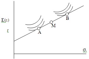
The CAPM model is applied generally in finance to determine a theoretically appropriate return of an asset. It presumes that investors must be compensated for investing in a risky asset in 2 ways – time value of money and risk itself. The beta term can be considered the “sensitivity” of the asset’s risk to market risk (both measured by variance). Consequently more “sensitive” assets ought to produce higher returns by CAPM. The graph below shows how asset return is linearly related to beta and that no beta implies a risk-free rate of return.
Apply for Hedge Fund Certification!
https://www.vskills.in/certification/certified-hedge-fund-manager