One of the important problems in inventory control is to balance the costs of holding inventories (holding costs) with the costs of placing orders for inventory replenishment (ordering costs). If a firm orders small quantities frequently its holding costs would be low but ordering costs will increase. On the other hand, in case the firm orders large quantities infrequently, its ordering costs will be low but holding costs would rise. A balance should be struck between the ordering costs and holding costs so as to minimize inventory costs. The EOQ (Economic Order quantity) approach is designed to achieve such a balance.
Economic order Quantity or optimum order quantity is that size of the order where total inventory costs (holding costs + ordering costs) are minimized. It is also known as “Economic Lot Size”.
The EOQ approach is based on the following assumptions.
- Inventory is consumed at a constant rate.
- Costs do not vary overtime.
- Lead Time is known and constant.
- Order costs, holding costs and unit price are constant.
- Holding costs are proportional to value of stocks held, similarly, order cost varies proportionately with price.
Total cost for managing inventory of an item depends upon 3 factors:
- Ordering cost (OC)
- Inventory Carrying Cost (ICC)
- Quantity Discounts (QD)
Ordering cost is the cost of placing one order. Total ordering cost per order can be determined by estimating annual cost actually incurred during the past one year against following elements:
- Salaries + Perks paid to all the employees in the purchase department
- Proportionate part of salary + perk of the executives and employees of other departments spending part of their time in making purchases. This will include accounts personnel associated with purchase department in evaluating quotations and making payments. Also QC department engaged in inspection and testing of purchased items
- Traveling expenses related to procurement
- Telephone, telegram, telex, postage and stationery relating to procurement
- Depreciation of accommodation (or rent of building) and equipment used for procurement.
- Insurance, power, water and other service charges relating to purchase department
- Any other cost (entertainment etc.) incurred for purchasing
If N is the number of orders placed during the year, ordering cost
| (S) in Rs. / Order = | Total Ordering Cost/Year N |
Inventory Carrying Cost (ICC): Inventory carrying cost is the cost of holding inventory. Various elements of cost falling under this head are as given below: –
- Interest loss/opportunity loss on the capital locked up in the form of average inventory.
- Salaries and perks of the employees engaged in the stores.
- Depreciation of accommodation (or rent of building) occupied by stored and stores offices.
- Depreciation of handling equipment, racks, furniture and other facilities used in stores.
- Obsolescence of items in stores.
- Deterioration, damage and pilferage of items during storage.
- Telephone, telex, postage and stationery used by stores.
- Handling expenses paid to contractors, transporters, etc.
- Insurance and taxes on stores.
- Electricity, oil, water and other service charges of stores.
- Any other cost relating to holding of stocks in the stores.
The method of calculating ICC is to estimate cost against each one of the above elements during the past year and divide it with the average inventory during that year. Average inventory can be calculated as follows: –
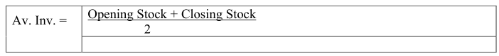
A better estimate of average inventory can be made by adding stock balance on the last day of each month of the previous year and dividing it by 12.
Let us take an example to explain the method of calculating ICC. If the stock balance on the last day of each month for previous year is 4, 4.5, 3, 6, 5, 4.5, 4, 4.5, 5.5,3,3,3 lakhs then
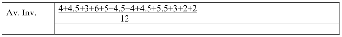
= 4 Lakhs
If the bank interest on working capital is 18% and total inventory holding cost against all elements listed from (ii) to (ix) above is Rs. 40,000 then

= 0.18 + 0.1
= 0.28 or 28% of Av. Inv.
The I.C.C. has a straight line relationship with the average inventory as shown in figure 8.2
Economic order quantity is defined as the order quantity against which total of OC and ICC is minimum. As shown in figure EOQ will be the order quantity where both ICC and OC curves interest each other. Mathematically this quantity is calculated by the following formula: –
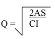
Where
Q = EOQ
A = Annual Consumption of the item in units.
S = Ordering Cost in Rs.
I = Inventory carrying cost as a fraction of the Iv. Inv.
C = Unit cost of the item in Rs.
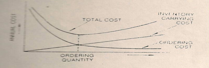
Figure 8.2
Let us say that during the next year forecast of consumption of an item is 5,000 units, S and I calculated on the basis of last year data are Rs. 50/- and 0.25 respectively and the unit price of the item is Rs. 2 then
If we assume the ordering cost S = 10 and the inventory carrying cost I = 20 percent or 0.20, for everyday use it is possible to workout EOQ data for different levels of annual consumption. It is not necessary to calculate the EOQ for each and every item, since the ordering cost and carrying cost vary only with number or orders and the value of purchase and not with the nature of the item to be purchased. An illustrative table incorporating economic order quantity and cost data for seven values of annual usage is given in table below: –
(EOQ data with = Rs. 10 per order and I = 20 percent or 0.20)
| Annual-Usage (A) Rs. | Economic Order Quantity (Q) Rs. | Time Supply | Number of Orders Per Year (A/Q) |
| 40,000 | 2,000 | 100 | 20 |
| 10,000 | 1,000 | 5 weeks | 10 |
| 8,100 | 900 | 6 weeks | 9 |
| 4,900 | 700 | 7.5 weeks | 7 |
| 1,600 | 400 | 3 months | 4 |
| 900 | 300 | 4 months | 3 |
| 100 | 100 | 1 Year | 1 |
From the table it can be easily seen that for C items, the cost of carrying inventory is naturally small and, for minimizing total cost, the ordering cost has to be kept low and so these items are ordered as in frequently as once or twice a year. On the other hand, for A items the inventory – carrying cost is high and for minimum total cost, the ordering cost should be very nearly equal to it. This means that the number of orders should be greater and purchases should be made more frequently in small lots so that inventories may be carried at a low level and at a low total cost
While, normally, purchases should be guided by the EOQ data similar to that shown above, departures can be made for god and valid reasons. The practical order quantity may be slightly more or less than that the critically calculated. It should be noted that the total cost curve is flat at the bottom and the total cost is therefore relatively insensitive over an appreciable range around the theoretically calculated quantity.
