
Microsoft Excel provides several ways to summarize values on your worksheet. You can create formulas that summarize data in columns, use tools that generate reports that summarize data in lists and it allows you to interactively change the view of the data.
Subtotals
Microsoft Excel can automatically calculate subtotal and grand total values in a list. When you insert automatic subtotals, Excel outlines the list so that you can display and hide the detail rows for each subtotal.

To insert subtotals, you first sort your list so that the rows you want to subtotal are grouped together. You can then calculate subtotals for any column that contains numbers. If your data isn’t organized as a list, or you only need a single total, you can use AutoSum instead of automatic subtotals.
How subtotals are calculated
- Subtotals Excel calculates subtotal values with a summary function, such as Sum or Average. You can display subtotals in a list with more than one type of calculation at a time.
- Grand totals Grand total values are derived from detail data, not from the values in the subtotal rows. For example, if you use the Average summary function, the grand total row displays an average of all detail rows in the list, not an average of the values in the subtotal rows.
- Automatic recalculation Excel recalculates subtotal and grand total values automatically as you edit the detail data.
Nesting subtotals
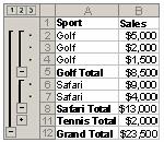
You can insert subtotals for smaller groups within existing subtotal groups. In the example below, subtotals for each sport are in a list that already has subtotals for each region.

- Outer subtotals 2. Nested subtotals
Before inserting nested subtotals, be sure to sort the list by all the columns for which you want subtotal values, so that the rows you want subtotaled are grouped together.
Summary reports and charts
Create summary reports – When you add subtotals to a list, the list is outlined so that you can see its structure. You can create a summary report by clicking the outline symbols , , and to hide the details and show only the totals.


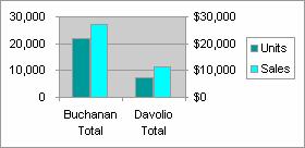
Chart the summary data – You can create a chart that uses only the visible data in a list that contains subtotals. If you show or hide details in the outlined list, the chart is also updated to show or hide the data.

Insert individual subtotals
- Make sure the data you want to subtotal is in the following format: each column has a label in the first row and contains similar facts, and there are no blank rows or columns within the range.
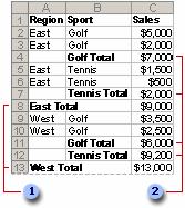
- Click a cell in the column to subtotal. In the example above, you’d click a cell in the Sport column, column B.
- Click Sort Ascending or Sort Descending .
- On the Data menu, click Subtotals.
- In the At each change in box, click the column to subtotal. In the example above, you’d click the Sport column.
- In the Use function box, click the summary function you want to use to calculate the subtotals.
- In the Add subtotal to box, select the check box for each column that contains values you want to subtotal. In the example above, you’d select the Sales column.
- If you want an automatic page break after each subtotal, select the Page break between groups check box.
- If you want the subtotals to appear above the subtotaled rows instead of below, clear the Summary below data check box.
- Click OK.
You can use the Subtotals command again to add more subtotals with different summary functions. To avoid overwriting the existing subtotals, clear the Replace current subtotals check box. To display a summary of just the subtotals and grand totals, click the outline symbols next to the row numbers. Use the and symbols to display or hide the detail rows for individual subtotals.
Insert nested subtotals
- Make sure the data you want to subtotal is in the following format: each column has a label in the first row and contains similar facts, and there are no blank rows or columns within the range.
- Sort the range by multiple columns, sorting first by the outer subtotal column, then by the next inner column for the nested subtotals, and so on. In the example above, you’d sort the range first by the Region column, and then by the Sport column.
- For best results, the range you sort should have column labels.
- Click a cell in the range you want to sort.
- On the Data menu, click Sort.
- In the Sort by and Then by boxes, click the columns you want to sort.
- Select any other sort options you want, and then click OK.
- Insert the outer subtotals.
- On the Data menu, click Subtotals.
- In the At each change in box, click the column for the outer subtotals. In the example above, you’d click Region.
- In the Use function box, click the summary function you want to use to calculate the subtotals.
- In the Add subtotal to box, select the check box for each column that contains values you want to subtotal. In the example above, that column would be Sales.
- If you want an automatic page break after each subtotal, select the Page break between groups check box.
- If you want the subtotals to appear above the subtotaled rows instead of below, clear the Summary below data check box.
Insert the nested subtotals.
- On the Data menu, click Subtotals.
- In the At each change in box, click the nested subtotal column. In the example above, that column would be Sport.
- Select the summary function and other options.
- Clear the Replace current subtotals check box.
Repeat the previous step for more nested subtotals, working from the outermost subtotals in.
Inserting and formatting a Summary Worksheet
When data is in list form, Microsoft Excel can create an outline to let you hide or show levels of detail with a single mouse click. An outline lets you quickly display only the rows or columns that provide summaries or headings for sections of your worksheet, or display the areas of detail data adjacent to a summary row or column.
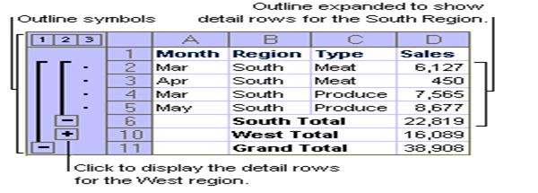
Displaying and hiding detail data – An outline can have up to eight levels of detail, with each inner level providing details for the preceding outer level. In the following example, the row containing the grand total of all the rows is level 1, the rows containing totals for the South and West regions are level 2, and the detail rows for the regions are level 3. To display only the rows for a particular level, you can click the number for the level you want to see. The detail rows for the West region are hidden, but you can click the + outline symbols to display the detail rows. As shown in the figure

Ways to outline data
Inserting automatic subtotals also creates an outline. If you use the Subtotal command in Data menu, to add subtotals to a list organized in rows, Excel outlines the worksheet so that you can show or hide as much detail as you need.
Outlining a worksheet automatically – If you have summarized data by using formulas that contain functions, such as SUM, Excel can automatically outline the data, as in the preceding example. The summary data must be adjacent to the detail data.
Outlining a worksheet manually – If the data is not organized so that Excel can outline it automatically, you can create an outline manually. For example, you’ll need to manually outline data if the rows or columns of summary data contain values instead of formulas, such as in the example below. If you want to hide the detail rows for April and May, you can do so by outlining the list manually.