
Basic probability concepts and terminology is discussed below
- Probability – It is the chance that something will occur. It is expressed as a decimal fraction or a percentage. It is the ratio of the chances favoring an event to the total number of chances for and against the event. The probability of getting 4 with a rolling of dice, is 1 (count of 4 in a dice) / 6 = .01667. Probability then can be the number of successes divided by the total number of possible occurrences. Pr(A) is the probability of event A. The probability of any event (E) varies between 0 (no probability) and 1 (perfect probability).
- Sample Space – It is the set of possible outcomes of an experiment or the set of conditions. The sample space is often denoted by the capital letter S. Sample space outcomes are denoted using lower-case letters (a, b, c . . .) or the actual values like for a dice, S={1,2,3,4,5,6}
- Event – An event is a subset of a sample space. It is denoted by a capital letter such as A, B, C, etc. Events have outcomes, which are denoted by lower-case letters (a, b, c . . .) or the actual values if given like in rolling of dice, S={1,2,3,4,5,6}, then for event A if rolled dice shows 5 so, A ={5}. The sum of the probabilities of all possible events (multiple E’s) in total sample space (S) is equal to 1.
- Independent Events – Each event is not affected by any other events for example tossing a coin three times and it comes up “Heads” each time, the chance that the next toss will also be a “Head” is still 1/2 as every toss is independent of earlier one.
- Dependent Events – They are the events which are affected by previous events like drawing 2 Cards from a deck will reduce the population for second card and hence, it’s probability as after taking one card from the deck there are less cards available as the probability of getting a King, for the 1st time is 4 out of 52 but for the 2nd time is 3 out of 51.
- Simple Events – An event that cannot be decomposed is a simple event (E). The set of all sample points for an experiment is called the sample space (S).
- Compound Events – Compound events are formed by a composition of two or more events. The two most important probability theorems are the additive and multiplicative laws.
- Union of events – The union of two events is that event consisting of all outcomes contained in either of the two events. The union is denoted by the symbol U placed between the letters indicating the two events like for event A={1,2} and event B={2,3} i.e. outcome of event A can be either 1 or 2 and of event B is 2 or 3 then, AUB = {1,2}
- Intersection of events – The intersection of two events is that event consisting of all outcomes that the two events have in common. The intersection of two events can also be referred to as the joint occurrence of events. The intersection is denoted by the symbol ∩ placed between the letters indicating the two events like for event A={1,2} and event B={2,3} then, A∩B = {2}
- Complement – The complement of an event is the set of outcomes in the sample space that are not in the event itself. The complement is shown by the symbol ` placed after the letter indicating the event like for event A={1,2} and Sample space S={1,2,3,4,5,6} then A`={3,4,5,6}
- Mutually Exclusive – Mutually exclusive events have no outcomes in common like the intersection of an event and its complement contains no outcomes or it is an empty set, Ø for example if A={1,2} and B={3,4} and A ∩ B= Ø.
- Equally Likely Outcomes – When a sample space consists of N possible outcomes, all equally likely to occur, then the probability of each outcome is 1/N like the sample space of all the possible outcomes in rolling a die is S = {1, 2, 3, 4, 5, 6}, all equally likely, each outcome has a probability of 1/6 of occurring but, the probability of getting a 3, 4, or 6 is 3/6 = 0.5.
- Probabilities for Independent Events or multiplication rule – Independent events occurrence does not depend on other events of sample space then the probability of two events A and B occurring both is P(A ∩ B) = P(A) x P(B) and similarly for many events the independence rule is extended as P(A∩B∩C∩. . .) = P(A) x P(B) x P(C) . . . This rule is also called as the multiplication rule. For example the probability of getting three times 6 in rolling a dice is 1/6 x 1/6 x 1/6 = 0.00463
- Probabilities for Mutually Exclusive Events or Addition Rule – Mutually exclusive events do not occur at the same time or in the same sample space and do not have any outcomes in common. Thus, for two mutually exclusive events, A and B, the event A∩B = Ø, and the probability of events A and B occurring is zero, as P(A∩B) = 0, for events A and B, the probabilities of either or both of the events occurring is P(AUB) = P(A) + P(B) – P(A∩B) also called as addition rule.For example let P(A) = 0.2, P(B) = 0.4, and P(A∩B) = 0.5, then P(AUB) = P(A) + P(B) – P(A∩B) = 0.2 + 0.4 – 0.5 = 0.1
- Conditional probability – It is the result of an event depending on the sample space or another event. The conditional probability of an event (the probability of event A occurring given that event B has already occurred) can be found as

For example in sample set of 100 items received from supplier1 (total supplied= 60 items and reject items = 4) and supplier 2(40 items), event A is the rejected item and B be the event if item from supplier1. Then, probability of reject item from supplier1 is – P(A|B) = P(A∩B)/ P(B), P(A∩B) = 4/100 and P(B) = 60/100 = 1/15.
It is important to have a computer analog of rolling a die. This is done on the computer by means of a random number generator. Depending upon the particular software package, the computer can be asked for a real number between 0 and 1, or an integer in a given set of consecutive integers. In the first case, the real numbers are chosen in such a way that the probability that the number lies in any particular subinterval of this unit interval is equal to the length of the subinterval. In the second case, each integer has the same probability of being chosen.
.203309 .762057 .151121 .623868
.932052 .415178 .716719 .967412
.069664 .670982 .352320 .049723
.750216 .784810 .089734 .966730
.946708 .380365 .027381 .900794
Let X be a random variable with distribution function m(ω), where ω is in the set {ω1, ω2, ω3}, and m(ω1) = 1/2, m(ω2) = 1/3, and m(ω3) = 1/6. If our computer package can return a random integer in the set {1, 2, …, 6}, then it is simply asked to do so, and make 1, 2, and 3 correspond to ω1, 4 and 5 correspond to ω2, and 6 correspond to ω3. If the computer package returns a random real number r in the interval (0, 1), then the expression
[6r] + 1will be a random integer between 1 and 6. (The notation [x] means the greatest integer not exceeding x, and is read “floor of x.”)
Probability Distributions
Prediction and decision-making needs fitting data to distributions (like normal, binomial, or Poisson). A probability distribution identifies whether a value will occur within a given range or the probability that a value that is lesser or greater than x will occur or the probability that a value between x and y will occur.
A distribution is the amount of variation in the outputs of a process, expressed by shape (symmetry, skewness and kurtosis), average and standard deviation. Symmetrical distributions the mean represents the central tendency of the data but for skewed distributions, the median is the indicator. The standard deviation provides a measure of variation from the mean. Similarly skewness is a measure of the location of the mode relative to the mean thus, if mode is to the mean’s left then the skewness is negative else positive but for symmetrical distribution, skewness is zero. Kurtosis measures the peakness or relative flatness of the distribution and the kurtosis is higher for a higher and narrower peak.
Probability distribution is a mathematical formula relating the values of a characteristic or attribute with their probability of occurrence in the population. It depicts the possible events and the associated probability for each of these events to occur. Probability distribution is divided as
- Discrete data describe a finite set of possible occurrences for the data like rolling a dice with the random variable can take value from 1, 2, 3, 4, 5 or 6. The most used discrete probability distributions are the binomial, the Poisson, the geometric, and the hypergeometric distribution.
- Continuous data describes a continuum of possible occurrences that is unbroken as, the distribution of body weight is a random variable with infinite number of possible data points.
Probability distributions for continuous variables use probability density functions (or PDF), which are mathematically model the probability density shown in a histogram but, discrete variables have probability mass function. PDFs employ integrals as the summation of area between two points when used in a equation. If a histogram shows the relative frequencies of a series of output ranges of a random variable, then the histogram also depicts the shape of the probability density for the random variable hence, the shape of the probability density function is also described as the shape of the distribution. An example illustrates it
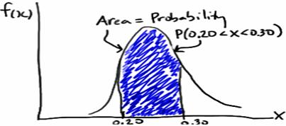
Example: A fast-food chain advertises a burger weighing a quarter-kg but, it is not exactly 0.25 kg. One randomly selected burger might weigh 0.23 kg or 0.27 kg. What is the probability that a randomly selected burger weighs between 0.20 and 0.30 kg? That is, if we let X denote the weight of a randomly selected quarter-kg burger in kg, what is P(0.20 < X < 0.30)?
This problem is solved by using probability density function as, imagine randomly selecting, 100 burgers advertised to weigh a quarter-kg. If weighed the 100 burgers, and created a density histogram of the resulting weights, perhaps the histogram might be

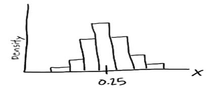
In this case, the histogram illustrates that most of the sampled burgers do indeed weigh close to 0.25 kg, but some are a bit more and some a bit less. Now, what if we decreased the length of the class interval on that density histogram then, it will be as

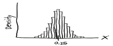
Now, if it is pushed further and the interval is decreased then, the intervals would eventually get small that we could represent the probability distribution of X, not as a density histogram, but rather as a curve (by connecting the “dots” at the tops of the tiny rectangles) as

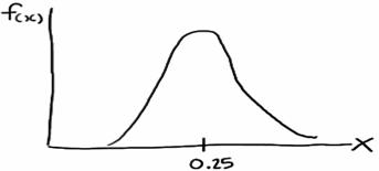
Such a curve is denoted f(x) and is called a (continuous) probability density function. A density histogram is defined so that the area of each rectangle equals the relative frequency of the corresponding class, and the area of the entire histogram equals 1. Thus, finding the probability that a continuous random variable X falls in some interval of values involves finding the area under the curve f(x) sandwiched by the endpoints of the interval. In the case of this example, the probability that a randomly selected burger weighs between 0.20 and 0.30 kg is then this area, as

Various distributions are
- Binomial – It is used in finite sampling problems when each observation has only one of two possible outcomes, such as pass/fail.
- Poisson – It is used for situations when an attribute possibility is that each sample can have multiple defects or failures.
- Normal – It is characterized by the traditional “bell-shaped” curve, the normal distribution is applied to many situations with continuous data that is roughly symmetrical around the mean.
- Chi-square – It is used in many situations when an inference is drawn on a single variance or when testing for goodness of fit or independence. Examples of use of this distribution include determining the confidence interval for the standard deviation of a population or comparing the frequency of variables.
- Student’s t – It is used in many situations when inferences are drawn without a variance known in the case of a single mean or the comparison of two means.
- F – It is used in situations when inferences are drawn from two variances such as whether two population variances are different in magnitude.
- Hypergeometric – It is the “true” distribution. It is used in a similar manner to the binomial distribution except that the sample size is larger relative to the population. This distribution should be considered whenever the sample size is larger than 10% of the population. The hypergeometric distribution is the appropriate probability model for selecting a random sample of n items from a population without replacement and is useful in the design of acceptance-sampling plans.
- Bivariate – It is created with the joint frequency distributions of modeled variables.
- Exponential – It is used for instances of examining the time between failures.
- Lognormal – It is used when raw data is skewed and the log of the data follows a normal distribution. This distribution is often used for understanding failure rates or repair times.
- Weibull – It is used when modeling failure rates particularly when the response of interest is percent of failures as a function of usage (time).