
Fixed overhead represents all items of expenditure which are more or less remain constant irrespective of the level of output or the number of hours worked.
Classification of Fixed Overhead Variances

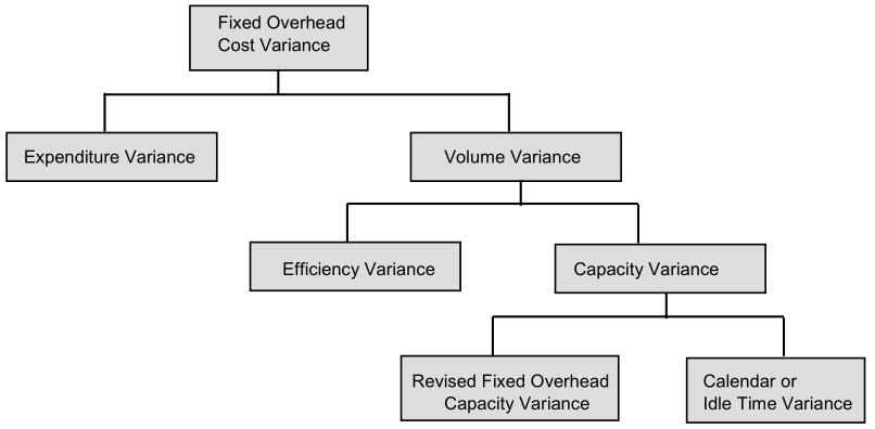
Fixed Overhead Cost Variance
Fixed overhead cost variance is the difference between the standard costs of fixed overhead allowed for the actual output achieved and the actual fixed overhead cost incurred i.e.
FOCV= (Actual output × Standard fixed overhead rate) – Actual fixed overheads
OR
(Standard hours produced × Standard fixed overhead rate per hour) – Actual fixed overheads
OR
Recovered fixed overhead – Actual fixed Overhead
Standard overhead produced means hours which should have been taken for the actual output
Fixed overhead variance may broadly be divided into:
- Expenditure variance and
- Volume variance.
Expenditure Variance
This is also known as budget variance. This is obtained by comparing the total overhead cost actually incurred against the budgeted overhead cost i.e.
Budgeted fixed overhead – Actual fixed overhead
OR
(Budgeted hours × Std. fixed overhead rate) – Actual fixed overhead
If the actual overheads are more, it shall result in an adverse variance and vice versa. This variance gives a measure of efficiency of spending.
Volume Variance
The difference between overhead absorbed on actual output and those on budgeted output is termed as volume variance. This variance shows the over or under absorption of fixed overheads during a particular period. If the actual output is more than the standard output, there is over-recovery of fixed overheads and volume variance is favorable and vice versa if the actual output is less than the standard output.
Volume Variance (FOVV) = (Actual output × Standard rate) – Budgeted fixed overheads OR
Standard rate (Actual output – Standard output) OR
Standard rate per hour (Standard hours produced – Budgeted hours) OR
(Absorbed overhead – Budgeted overhead)
N.B: Standard hour produced means number of hours which should have been taken for the actual output as per the standard lay down.
Verify: F.O. COST VARIANCE = F.O. EXPENDITURE VARIANCE + F.O. VOLUME VARIANCE
Volume variance can be further sub-divided into the following variances:
Efficiency Variance: It arises due to the difference between the output actually achieved and the output which should have been achieved in the actual hours worked. This variance will be favorable it the actual production is more than the standard production in actual hours.
Fixed Overhead Efficiency Variance (FOEfV)=
Standard Fixed Overhead Rate per hour [Standard Production – Actual Production]
Capacity Variance: It is that portion of the volume variance which is due to working at higher or lower capacity than the standard capacity. It is related to the under or over utilization of plant and equipment. If the capacity utilization is more than the budgeted capacity, the variance is favorable, otherwise it will be adverse. It is represented as:
F. O. Capacity Variance= Standard rate (Standard quantity – Budgeted quantity)
Revised Capacity Variance: This variance indicates the difference in capacity utilization due to working for more or less number of days than the budgeted one. The computation of this variance is done by using the following formula.
Fixed Overhead Revised Capacity Variance (FORCV) = Standard Rate [Standard Quantity – Revised Budgeted Quantity]
Calendar (Idle Time) Variance: It is that portion of the volume variance which is due to the difference between the number of working days anticipated in the budget period and the actual working days in the period to which the budget is applied. If the actual working days exceed standard days, the variance will be favorable and vice-versa.
It is calculated as:
FO Calendar Variance = Standard rate (Revised budgeted units – Budgeted units)
OR
Increase or decrease in production due to more or less working days at the rate of revised capacity × Standard rate per unit.
Illustration 5
The budgeted capacity of a factory per month of 25 days was 2,00,000 hours and the budgeted fixed overheads were 2,40,000. The management increased the capacity by 20% in the beginning of October, 2000, the actual number of working days in that month were 23. Compute the variance that emerges.
Solution:
Budgeted fixed overheads recovery rate 1.20 i.e. 2,40,000/2,00,000.
Actual production in terms of hours (2,00,000 + 20%) × 23/25 or 2,20,800
Volume Variance:
Fixed overheads absorbed on 2,20,800
hours @ 1.20 per hours 2,64,960
Budgeted fixed overheads 2,40,000
Volume Variance 24,960 (F)
(or 20,800 hours @ 1.20)

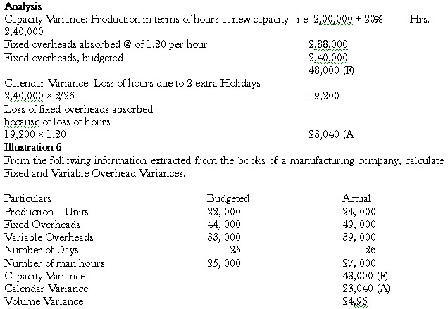
Solution:
(A) Fixed Overhead Variances:
(I) Fixed Overhead Cost Variance:
Standard Fixed Overheads for Actual Production – Actual Fixed Overheads
= 48, 000 – 49, 000 = 1, 000 [A]
Note: Standard fixed overheads for actual production = Actual Production 24, 000 × standard rate 2 [44, 000 budgeted fixed overheads / 22, 000 budgeted production = 2]
(II) Fixed Overhead Expenditure Variance
Budgeted Fixed Overheads – Actual Fixed Overheads
= 44, 000 – 49, 000 = 5, 000 [A]
(III) Fixed Overhead Volume Variance
Standard Rate [Budgeted Quantity – Actual Quantity] =
2 [22, 000 – 24, 000] = 4, 000 [F]
The variance is favorable as the actual quantity produced is more than the budgeted quantity.
Reconciliation I = Cost Variance = Expenditure Variance + Volume Variance
1, 000 [A] = 5, 000 [A] + 4, 000 [F]
(IV) Fixed Overhead Efficiency Variance
Standard Rate [Standard Quantity – Actual Quantity] = 2 [23, 760 – 24, 000] = 480 [F]
Note: Standard quantity of production is in reference to actual number of hours. If 22, 000 units are produced in 25, 000 hrs [standard hours], in actual 27, 000 hours, 23, 760 units should have been produced. When number of days and number of hours, both are given, the standard quantity is always to be computed in relation to the actual hours. However, if only number of days is given, the standard quantity will have to be computed in relation to number of days.
(V) Fixed Overhead Capacity Variance
Standard Rate [Standard Quantity – Budgeted Quantity] = 2 [23, 760 – 22, 000] = 3, 520 [F]
Reconciliation II = Volume Variance = Efficiency Variance + Capacity Variance
4, 000 [F] = 480 [F] + 3, 520 [F]
(VI) Fixed Overhead Revised Capacity Variance
= Standard Rate [Standard Quantity – Revised Budgeted Quantity]
= 2 [23,760 – 22,880] = 2 × 880 = 1760 [F]
Note: Standard quantity is computed as shown in the Efficiency Variance. Revised Budget Quantity is computed as: in 25 days, the production is 22,000 so in 26 days the revised quantity is 22,880 units.
(VII) Fixed Overhead Calendar Variance
Standard Rate [Revised Budgeted Quantity – Budgeted Quantity]
= 2 [22,880 – 22,000] = 2 × 880 = 1,760 [F]
Reconciliation III = Capacity Variance = Revised Capacity Variance + Calendar Variance =
3, 520 [F] = 1760 [F] + 1760 [F] = 367
(I) Cost Variance: Standard Variable Overheads for Actual Production – Actual Variable Overheads:
36,000 – 39,000 = 3,000 [A]
Note: Standard Variable Overheads for Actual Production = Standard Rate Per Unit × Actual Production Units = 1.5 [Budgeted variable overheads 33,000 /Budgeted production units
22,000 = 1.5] × 24,000 units = 36,000
(II) Expenditure Variance: Standard Variable Overheads for Standard Production – Actual Variable Overheads: 1.5 × 23, 760 – 39,000 = 3360 [A]
(III) Efficiency Variance: Standard Rate [Standard Quantity – Actual Quantity]
1.5 [23,760 – 24,000] = 360 [F]