
What does your data tell you? Analysis is often intertwined with the data collection and measurement. The data collection team may consist of different people who will collect different sets of data or additional data. As the team reviews the data collected, they may decide to adjust the data collection plan to include additional information. This continues as the team analyzes both the data and the process to narrow down and verify the root causes of waste and defects.
Data analysis is the study and understanding of variables in a process, for example leading to the outcome of an experiment. To support data analysis, you need numerical x values. These x value inputs lead to the variable y outputs for the process. The values can be continuous or discrete.
In addition, you need to understand the range represented by the probability distribution. For example, Process A, B, and C on a line chart can each have different ranges of probability distribution.
A probability distribution lists the outcomes of an experiment. By doing so, it helps link what each outcome is and its probability of occurrence in that population of data in future. It also assists in data analysis and decision making, to help you understand whether you’ll be doing the right thing at the right time in future.
It is a mathematical formula relating the values of a characteristic or attribute with their probability of occurrence in the population. It depicts the possible events and the associated probability for each of these events to occur. Probability distribution is divided as
- Discrete data describe a finite set of possible occurrences for the data like rolling a dice with the random variable can take value from 1, 2, 3, 4, 5 or 6. The most used discrete probability distributions are the binomial, the Poisson, the geometric, and the hypergeometric distribution.
- Continuous data describes a continuum of possible occurrences that is unbroken as, the distribution of body weight is a random variable with infinite number of possible data points.
Probability Density Function
Probability distributions for continuous variables use probability density functions (or PDF), which are mathematically model the probability density shown in a histogram but, discrete variables have probability mass function. PDFs employ integrals as the summation of area between two points when used in an equation. If a histogram shows the relative frequencies of a series of output ranges of a random variable, then the histogram also depicts the shape of the probability density for the random variable hence, the shape of the probability density function is also described as the shape of the distribution. An example illustrates it
Example: A fast-food chain advertises a burger weighing a quarter-kg but, it is not exactly 0.25 kg. One randomly selected burger might weigh 0.23 kg or 0.27 kg. What is the probability that a randomly selected burger weighs between 0.20 and 0.30 kg? That is, if we let X denote the weight of a randomly selected quarter-kg burger in kg, what is P(0.20 < X < 0.30)?
This problem is solved by using probability density function as, imagine randomly selecting, 100 burgers advertised to weigh a quarter-kg. If weighed the 100 burgers, and created a density histogram of the resulting weights, perhaps the histogram might be

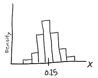
In this case, the histogram illustrates that most of the sampled burgers do indeed weigh close to 0.25 kg, but some are a bit more and some a bit less. Now, what if we decreased the length of the class interval on that density histogram then, it will be as

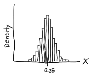
Now, if it is pushed further and the interval is decreased then, the intervals would eventually get small that we could represent the probability distribution of X, not as a density histogram, but rather as a curve (by connecting the “dots” at the tops of the tiny rectangles) as

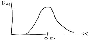
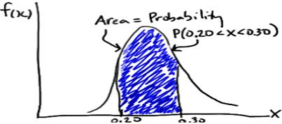
Such a curve is denoted f(x) and is called a (continuous) probability density function. A density histogram is defined so that the area of each rectangle equals the relative frequency of the corresponding class, and the area of the entire histogram equals 1. Thus, finding the probability that a continuous random variable X falls in some interval of values involves finding the area under the curve f(x) sandwiched by the endpoints of the interval. In the case of this example, the probability that a randomly selected burger weighs between 0.20 and 0.30 kg is then this area, as

Distributions Types
Various distributions are
- Binomial – It is used in finite sampling problems when each observation has only one of two possible outcomes, such as pass/fail.
- Poisson – It is used for situations when an attribute possibility is that each sample can have multiple defects or failures.
- Normal – It is characterized by the traditional “bell-shaped” curve, the normal distribution is applied to many situations with continuous data that is roughly symmetrical around the mean.
- Chi-square – It is used in many situations when an inference is drawn on a single variance or when testing for goodness of fit or independence. Examples of use of this distribution include determining the confidence interval for the standard deviation of a population or comparing the frequency of variables.
- Student’s t – It is used in many situations when inferences are drawn without a variance known in the case of a single mean or the comparison of two means.
- F – It is used in situations when inferences are drawn from two variances such as whether two population variances are different in magnitude.
- Hypergeometric – It is the “true” distribution. It is used in a similar manner to the binomial distribution except that the sample size is larger relative to the population. This distribution should be considered whenever the sample size is larger than 10% of the population. The hypergeometric distribution is the appropriate probability model for selecting a random sample of n items from a population without replacement and is useful in the design of acceptance-sampling plans.
- Bivariate – It is created with the joint frequency distributions of modeled variables.
- Exponential – It is used for instances of examining the time between failures.
- Lognormal – It is used when raw data is skewed and the log of the data follows a normal distribution. This distribution is often used for understanding failure rates or repair times.
- Weibull – It is used when modeling failure rates particularly when the response of interest is percent of failures as a function of usage (time).